Laser Microphone: Difference between revisions
Nicholas cjl (talk | contribs) |
Nicholas cjl (talk | contribs) |
||
| (80 intermediate revisions by 2 users not shown) | |||
| Line 8: | Line 8: | ||
A0171267A | [[User:Nicholas cjl|Nicholas Chong Jia Le]] | A0171267A | [[User:Nicholas cjl|Nicholas Chong Jia Le]] | ||
== | Some of the code and files used can be found on [https://github.com/NicholasCJL/PC5214 GitHub]. | ||
== Requirements == | |||
Using a photodiode / array of photodiodes, we attempt to record audio by measuring the signal from a laser reflecting off a surface near the sound. | Using a photodiode / array of photodiodes, we attempt to record audio by measuring the signal from a laser reflecting off a surface near the sound. | ||
Due to the nature of the setup mentioned, we require a decently dim environment to minimise noise, a visible light laser (does not need to be high powered but needs to be decently collimated), an optical bench, a set of photodiodes that can detect the laser light and produce a signal, and an electronic setup that allows us to capture and export the signal from the photodiodes. | Due to the nature of the setup mentioned, we require a decently dim environment to minimise noise, a visible light laser (does not need to be high powered but needs to be decently collimated), an optical bench, a set of photodiodes that can detect the laser light and produce a signal, and an electronic setup that allows us to capture and export the signal from the photodiodes. | ||
== Project Objectives == | |||
The following are the main objectives of our project keeping the experimental timeframe we had of about 8 weeks in mind. | |||
* Conceptualise a setup that can theoretically transmit audio information indirectly with a laser reflecting off a surface. | |||
* Demonstrate the ability to transmit some level of audio information with a laser with as little specialised equipment as possible. | |||
* Attempt simple filtering techniques to improve the signal obtained (at least to the human ear). | |||
If there is time, we will attempt the following additional objective. | |||
* Modify the setup to try to improve on the signal obtained so it is more intelligible, such that a person listening can identify the audio from the modified setup better compared to the original setup. | |||
== Background == | == Background == | ||
=== Level (logarithmic quantity) === | === Level (logarithmic quantity) === | ||
A power level is a logarithmic quantity used to measure power, power density or sometimes energy, with commonly used unit decibel (dB). | A power level is a logarithmic quantity used to measure power, power density or sometimes energy, with the commonly used unit decibel (dB). | ||
===Power level=== | |||
====Power level==== | |||
Level of a ''power'' quantity, denoted ''L''<sub>''P''</sub>, is defined by | Level of a ''power'' quantity, denoted ''L''<sub>''P''</sub>, is defined by | ||
:<math>L_P = \frac{1}{2} \log_{\mathrm{e}}\!\left(\frac{P}{P_0}\right)\!~\mathrm{Np} = \log_{10}\!\left(\frac{P}{P_0}\right)\!~\mathrm{B} = 10 \log_{10}\!\left(\frac{P}{P_0}\right)\!~\mathrm{dB}.</math> | :<math>L_P = \frac{1}{2} \log_{\mathrm{e}}\!\left(\frac{P}{P_0}\right)\!~\mathrm{Np} = \log_{10}\!\left(\frac{P}{P_0}\right)\!~\mathrm{B} = 10 \log_{10}\!\left(\frac{P}{P_0}\right)\!~\mathrm{dB}.</math> | ||
| Line 25: | Line 40: | ||
*''P''<sub>0</sub> is the reference value of ''P''. | *''P''<sub>0</sub> is the reference value of ''P''. | ||
===Field (or root-power) level=== | ====Field (or root-power) level==== | ||
The level of a ''root-power'' quantity (also known as a ''field'' quantity), denoted ''L''<sub>''F''</sub>, is defined by | The level of a ''root-power'' quantity (also known as a ''field'' quantity), denoted ''L''<sub>''F''</sub>, is defined by | ||
:<math>L_F = \log_{\mathrm{e}}\!\left(\frac{F}{F_0}\right)\!~\mathrm{Np} = 2 \log_{10}\!\left(\frac{F}{F_0}\right)\!~\mathrm{B} = 20 \log_{10}\!\left(\frac{F}{F_0}\right)\!~\mathrm{dB}.</math> | :<math>L_F = \log_{\mathrm{e}}\!\left(\frac{F}{F_0}\right)\!~\mathrm{Np} = 2 \log_{10}\!\left(\frac{F}{F_0}\right)\!~\mathrm{B} = 20 \log_{10}\!\left(\frac{F}{F_0}\right)\!~\mathrm{dB}.</math> | ||
| Line 31: | Line 46: | ||
*''F'' is the root-power quantity, proportional to the square root of power quantity; | *''F'' is the root-power quantity, proportional to the square root of power quantity; | ||
*''F''<sub>0</sub> is the reference value of ''F''. | *''F''<sub>0</sub> is the reference value of ''F''. | ||
[https://en.wikipedia.org/wiki/Sound_pressure Sound pressure] is a root power quantity, and thus uses this definition of the decibel. | |||
=== Low-pass filter === | === Low-pass filter === | ||
| Line 58: | Line 75: | ||
<gallery widths= | <gallery widths=470px heights=340px> | ||
File:NMLMbworth filter gain.png|Plot of the (power) gain <math>G(f)</math> vs log frequency <math>\log_{10}f</math> of low-pass Butterworth filters of different orders with cutoff frequency <math>f=1</math> Hz, showing the increasing rate of frequency rejection as the order of the filters increase. Green dotted line marks cutoff frequency <math>f_c = 1</math> Hz. | File:NMLMbworth filter gain.png|Plot of the (power) gain <math>G(f)</math> vs log frequency <math>\log_{10}f</math> of low-pass Butterworth filters of different orders with cutoff frequency <math>f=1</math> Hz, showing the increasing rate of frequency rejection as the order of the filters increase. Green dotted line marks cutoff frequency <math>f_c = 1</math> Hz. | ||
File:NMLMbworth filter gain zoomed.png|Plot of the gain <math>G(f)</math> vs log frequency <math>\log_{10}f</math> of different order low-pass Butterworth filters with the cutoff point magnified, showing increasing sharpness in the cutoff behaviour as the order of the filters increase. Green dotted line marks cutoff frequency <math>f_c = 1</math> Hz. | File:NMLMbworth filter gain zoomed.png|Plot of the gain <math>G(f)</math> vs log frequency <math>\log_{10}f</math> of different order low-pass Butterworth filters with the cutoff point magnified, showing increasing sharpness in the cutoff behaviour as the order of the filters increase. Green dotted line marks cutoff frequency <math>f_c = 1</math> Hz. | ||
| Line 89: | Line 106: | ||
The voltage measured should correspond almost directly to the envelope of the carrier wave if we use a visible light laser. This is because the frequency of visible light is in the hundreds of THz (~<math>10^{14}</math> to <math>10^{15}</math> Hz), while the cutoff frequency of the photodiode used<ref>Hamamatsu Photonics. [https://www.hamamatsu.com/content/dam/hamamatsu-photonics/sites/documents/99_SALES_LIBRARY/ssd/s5980_etc_kpin1012e.pdf ''Datasheet for S5980/S5981/S5870 series Si PIN photodiodes''] Jan 2021</ref> is on the order of <math>10^7</math> Hz. As such, the high frequency component of the carrier wave (laser) is effectively filtered out by the photodiode acting as a low-pass filter, leaving just the lower frequency amplitude modulation component in an ideal case. | The voltage measured should correspond almost directly to the envelope of the carrier wave if we use a visible light laser. This is because the frequency of visible light is in the hundreds of THz (~<math>10^{14}</math> to <math>10^{15}</math> Hz), while the cutoff frequency of the photodiode used<ref>Hamamatsu Photonics. [https://www.hamamatsu.com/content/dam/hamamatsu-photonics/sites/documents/99_SALES_LIBRARY/ssd/s5980_etc_kpin1012e.pdf ''Datasheet for S5980/S5981/S5870 series Si PIN photodiodes''] Jan 2021</ref> is on the order of <math>10^7</math> Hz. As such, the high frequency component of the carrier wave (laser) is effectively filtered out by the photodiode acting as a low-pass filter, leaving just the lower frequency amplitude modulation component in an ideal case. | ||
==Quality of Reproduced Audio== | |||
On top of just judging how close the reproduced audio is to the original audio by listening to it, we can use a second measure to objectively quantify the quality or "closeness" of the reproduced audio to the original. The [https://code.google.com/archive/p/musicg/ <code>musicg</code>] module was used, which contained a <code>fingerprint</code> package that allows the "fingerprinting" of audio files by obtaining the spectrogram at each sample interval. The same module also allows for the comparison of the fingerprints of both files, giving a similarity score <math>S_0</math>. The code for calculating similarity works as follows: | |||
# The audio files are split into "frames" based on the sample rate, | |||
# the spectrogram of each frame is calculated, | |||
# the files are "aligned" based on the alignment with the maximum "match" count between the two files, | |||
# the total number of matches is divided by the total number of frames to give a similarity score showing the number of matches per frame. | |||
The value of a "match" is calculated by the difference between the spectrograms in each frame, the more the spectrograms overlap, the greater the value of a match. The raw value of the similarity score is in arbitrary units that is consistent across different pairs of audio compared. In this project, we will treat a score of 1.0 (at least one "match" per frame) and above to be a perfect reproduction of the audio. Any score less than 1.0 represents a less than perfect reproduction of the audio. Because the code only looks for matches (score does not get deducted by lack of a match), this is a good way to quantify reproduction quality with small amounts of background noise being acceptable. | |||
The table below shows an example of the similarity score between 3 different audio files. | |||
{| class="wikitable" style="text-align:center;" | |||
|- | |||
! <math>S_0</math> | |||
! Pure 200 Hz tone | |||
! Pure 200 Hz tone + white noise | |||
! Pure 300 Hz tone | |||
! Pure 300 Hz tone + white noise | |||
|- | |||
| [https://soundcloud.com/laser-microphone/source-200hz Pure 200 Hz tone] | |||
| 3.35714 | |||
| style="background-color:#c0c0c0;" | - | |||
| style="background-color:#c0c0c0;" | - | |||
| style="background-color:#c0c0c0;" | - | |||
|- | |||
| [https://soundcloud.com/laser-microphone/source-200hz-noise Pure 200 Hz tone + white noise] | |||
| 0.63265 | |||
| 2.92857 | |||
| style="background-color:#c0c0c0;" | - | |||
| style="background-color:#c0c0c0;" | - | |||
|- | |||
| [https://soundcloud.com/laser-microphone/source-300hz Pure 300 Hz tone] | |||
| 0.0 | |||
| 0.0 | |||
| 3.35714 | |||
| style="background-color:#c0c0c0;" | - | |||
|- | |||
| [https://soundcloud.com/laser-microphone/source-300hz-noise Pure 300 Hz tone + white noise] | |||
| 0.02041 | |||
| 0.01020 | |||
| 0.67347 | |||
| 3.06122 | |||
|} | |||
===Difficulties=== | |||
Even though the module provided a way to quantify the similarity between two pieces of audio (something that is not trivial to do), we had to make some modifications to the source code. Due to the module being written for a depreciated version of Java from over a decade ago, it relies on libraries that are no longer supported. As such, we had to reimplement a small portion of the [https://en.wikipedia.org/wiki/Fast_Fourier_transform Fast Fourier Transform] algorithm within the source code, which took quite some time (as we are trained in Python, not Java!). After quite a bit of relearning Java, we managed to get the module and the functions required working. | |||
We found that with large levels of distortion and noise, this metric becomes significantly less useful as it cannot account for frequency shifts and large shifts in the dynamics of the audio. An example for the former would be two tracks that are slightly pitch shifted relative to each other which would be trivial for a human to indicate a high similarity score for, but this method will give a low similarity score for. An example of the latter would be a track with the volume of the low frequencies boosted significantly, which again would still keep a high similarity score when judged by a human, but will be poorly judged by this method as the code normalises the spectrograms before conducting the similarity check (causing some features to "disappear" if other features get too loud). This second effect will primarily be caused by resonance as we will observe later. We will see later on that other than for simple pure frequency comparisons, this metric is not a very good indicator of similarity due to the large amounts of distortion our setup introduces. The similarity scores will still be indicated, but the score will be <span style="color:#ff0000"> coloured red</span> to indicate that we do not think it is a reliable measure of similarity. | |||
For future reference, a similarity metric that uses something like computer vision to match features in the spectrograms or deep learning to identify spectrogram features might be more useful. | |||
==Original Setup== | ==Original Setup== | ||
| Line 96: | Line 167: | ||
The original setup was created with as few components as possible to create a baseline performance that we can compare to. A schematic of the setup is shown in the image above. A Melles Griot HeNe laser with a wavelength of 632.8 nm was used to function as the carrier wave. The laser impinges upon a mirror attached to a surface near a pair of speakers, then gets reflected onto a photodiode which is connected to an oscilloscope. The components are shown below. | The original setup was created with as few components as possible to create a baseline performance that we can compare to. A schematic of the setup is shown in the image above. A Melles Griot HeNe laser with a wavelength of 632.8 nm was used to function as the carrier wave. The laser impinges upon a mirror attached to a surface near a pair of speakers, then gets reflected onto a photodiode which is connected to an oscilloscope. The setup is aligned such that when the surface vibrates along with the mirror, an angular displacement of the laser beam occurs and there is a longitudinal displacement of the laser spot at the photodiode. The mirror and photodiode are separated by about 6 metres, so any small angular displacement results in a large longitudinal displacement and resulting shift in total power incident on the photodiode, changing the voltage output detected by the oscilloscope. This setup implements the amplitude modulation discussed previously by converting small physical motions to changes in the amplitude of the voltage recorded. The components are shown below. | ||
<gallery widths= | <gallery widths=300px heights=210px> | ||
File:NMLMpower_laser.jpg|Laser connected to power supply. | File:NMLMpower_laser.jpg|Laser connected to power supply. | ||
File:NMLMtube_mirror.jpg|Mirror mounted on original surface constructed with a balloon stretched over a 3D printed cylinder. | File:NMLMtube_mirror.jpg|Mirror mounted on original surface constructed with a balloon stretched over a 3D printed cylinder. | ||
| Line 108: | Line 179: | ||
Note that as seen in the photo of the photodiode, the laser is not centered on the photodiode but instead on one corner. We found that this improved the signal received, as this allowed small deflections to also be detected when the laser shifted in any direction, including towards the center of the photodiode (which increased the overall power on the photodiode). In contrast, if the laser is centered on the photodiode, small deflections will not be detected as the voltage output by the photodiode is only dependent on the total power received and not the location on its surface. | Note that as seen in the photo of the photodiode, the laser is not centered on the photodiode but instead on one corner. We found that this improved the signal received, as this allowed small deflections to also be detected when the laser shifted in any direction, including towards the center of the photodiode (which increased the overall power on the photodiode). In contrast, if the laser is centered on the photodiode, small deflections will not be detected as the voltage output by the photodiode is only dependent on the total power received and not the location on its surface. | ||
===Oscilloscope Settings=== | |||
The following settings were used for the oscilloscope: | |||
* 1 MΩ input impedance | |||
* 0.1 mV voltage resolution | |||
* 50 μs time resolution | |||
The choice of the time resolution was done as a compromise between the [https://en.wikipedia.org/wiki/Nyquist_frequency Nyquist frequency] placing a lower bound on the number of samples per second we can take, and wanting a reasonably long recording placing an upper bound on the number of samples per second (since the oscilloscope has a limited amount of memory to store recordings). Our current choice of 20 kilosamples per second gives a Nyquist frequency of 10 kHz, which should capture a decent frequency range for low quality recordings. This also gives us a 5 second long recording, which we decided was the minimum recording length which we can demonstrate the ability of our setup with. | |||
==Results (Original Setup)== | ==Results (Original Setup)== | ||
===Pure Frequencies=== | |||
We tested the original setup with pure tones as a proof of concept in order to determine if such a setup can transmit any information. The spectra of the different tones tested along with the audio reconstructed from the output of the receiver are seen in the table below. The red lines in each graph show the frequency of the test tone played. From the spectra and audio, it is clear that the concept works, and we are able to transmit audio information simply by reflecting a laser off a surface near the audio, and collecting the reflected beam with a photodiode, followed by recording the voltage output from the photodiode. A second order low-pass Butterworth filter was applied to each audio recording at 2000 Hz in order to remove the background noise. | |||
Even though we played pure frequencies, we see multiple spikes at integer multiples of those frequencies, indicating that the harmonics are also induced on the surface, which is expected and is a characteristic of the surface, also known as [https://en.wikipedia.org/wiki/Timbre timbre] in music. The average difference between the frequency in the reconstructed audio and the frequency transmitted <math>\Delta f_0</math> is also indicated in the table, showing small deviations between the reconstructed signal and the transmitted signal. | |||
We note that for some frequencies (300 Hz, 500 Hz), the audio obtained is not correct. This is because a higher harmonic was activated more strongly than the fundamental for those frequencies, causing the harmonics to be recorded instead. For 600 Hz and 700 Hz, barely any signal could be heard which is a function of both the weaker response of the vibrating surface to those frequencies, and our perception of volume being different for different frequencies. | |||
{| class="wikitable" style="text-align:center;" | |||
|- style="background-color:#c0c0c0;" | |||
! Transmitted Frequency | |||
! <math>P</math> vs <math>\log_{10}{f}</math> | |||
! <math>P</math> vs <math>f</math> | |||
! <math>P</math> vs <math>\log_{10}{f}</math> (Filtered) | |||
! <math>\Delta f_0</math> / Hz | |||
! Audio | |||
! <math>S_0</math> (source vs unfiltered) | |||
! <math>S_0</math> (source vs filtered) | |||
|- | |||
| 100 | |||
| [[File:NMLM100Hz_1.png|250px]] | |||
| [[File:NMLM100Hz_1_flat.png|250px]] | |||
| [[File:NMLM100Hz_1_filtered.png|250px]] | |||
| -0.04 <math>\pm</math> 0.13 | |||
| [https://soundcloud.com/laser-microphone/original-100hz-1 Unfiltered] vs [https://soundcloud.com/laser-microphone/original-100hz-1-filtered filtered] | |||
| 0.09184 | |||
| 0.15306 | |||
|- | |||
| 200 | |||
| [[File:NMLM200Hz_1.png|250px]] | |||
| [[File:NMLM200Hz_1_flat.png|250px]] | |||
| [[File:NMLM200Hz_1_filtered.png|250px]] | |||
| 0.8 <math>\pm</math> 2.3 | |||
| [https://soundcloud.com/laser-microphone/original-200hz-1 Unfiltered] vs [https://soundcloud.com/laser-microphone/original-200hz-1-filtered-1 filtered] | |||
| 0.64286 | |||
| 0.5 | |||
|- | |||
| 300 | |||
| [[File:NMLM300Hz_1.png|250px]] | |||
| [[File:NMLM300Hz_1_flat.png|250px]] | |||
| [[File:NMLM300Hz_1_filtered.png|250px]] | |||
| 0.08 <math>\pm</math> 0.14 | |||
| [https://soundcloud.com/laser-microphone/original-300hz-1 Unfiltered] vs [https://soundcloud.com/laser-microphone/original-300hz-1-filtered filtered] | |||
| <span style="color:#ff0000>0.0</span> | |||
| <span style="color:#ff0000>0.0</span> | |||
|- | |||
| 400 | |||
| [[File:NMLM400Hz_1.png|250px]] | |||
| [[File:NMLM400Hz_1_flat.png|250px]] | |||
| [[File:NMLM400Hz_1_filtered.png|250px]] | |||
| 0.32 <math>\pm</math> 0.28 | |||
| [https://soundcloud.com/laser-microphone/original-400hz-1 Unfiltered] vs [https://soundcloud.com/laser-microphone/original-400hz-1-filtered filtered] | |||
| 0.22449 | |||
| 0.18367 | |||
|- | |||
| 500 | |||
| [[File:NMLM500Hz_1.png|250px]] | |||
| [[File:NMLM500Hz_1_flat.png|250px]] | |||
| [[File:NMLM500Hz_1_filtered.png|250px]] | |||
| -0.07 <math>\pm</math> 0.15 | |||
| [https://soundcloud.com/laser-microphone/original-500hz-1 Unfiltered] vs [https://soundcloud.com/laser-microphone/original-500hz-1-filtered filtered] | |||
| 0.60204 | |||
| 0.66327 | |||
|- | |||
| 600 | |||
| [[File:NMLM600Hz_1.png|250px]] | |||
| [[File:NMLM600Hz_1_flat.png|250px]] | |||
| [[File:NMLM600Hz_1_filtered.png|250px]] | |||
| 1.6 <math>\pm</math> 3.6 | |||
| [https://soundcloud.com/laser-microphone/original-600hz-1 Unfiltered] vs [https://soundcloud.com/laser-microphone/original-600hz-1-filtered filtered] | |||
| 0.02040 | |||
| 0.19388 | |||
|- | |||
| 700 | |||
| [[File:NMLM700Hz_1.png|250px]] | |||
| [[File:NMLM700Hz_1_flat.png|250px]] | |||
| [[File:NMLM700Hz_1_filtered.png|250px]] | |||
| 0.07 <math>\pm</math> 0.14 | |||
| [https://soundcloud.com/laser-microphone/original-700hz-1 Unfiltered] vs [https://soundcloud.com/laser-microphone/original-700hz-1-filtered filtered] | |||
| 0.56122 | |||
| 0.68367 | |||
|} | |||
===Real-World Audio=== | |||
After testing the pure frequencies, we tested out two clips from a person speaking. We found that due to the response of our stretched balloon membrane being highly focused around the vibrational modes of the membrane, the transmitted signal is extremely distorted. Furthermore, we observed the phenomenon of [https://en.wikipedia.org/wiki/Clipping_(audio) clipping] when certain frequencies cause large amplitude vibrations in the membrane. As the photodiode has a minimum voltage output when the laser spot is completely off the photodiode corresponding to a certain vibrational amplitude, there is a limit to the vibrational amplitude it can capture, meaning any vibration above that amplitude gets flattened to that level. These "clipped" sections are not only much louder than the surrounding sections, they introduce huge amounts of distortion in the reconstructed audio as the clipped section approaches a square wave, introducing high frequency components not present in the original audio. | |||
==== Seashells ==== | |||
The first piece of audio used was a classic tongue twister found [https://soundcloud.com/laser-microphone/seashells-source here]. The images below show the raw voltage over time recorded, showing large audio clipping and transient asymmetry. After passing the audio through a 2nd order band-pass Butterworth filter with the passband from 100 Hz to 2000 Hz, the waveform looks significantly more like what we would expect from a normal audio waveform. This is because the asymmetry in the transient spikes correspond to high frequency components that are removed during the filtering. The recorded audio can be found [https://soundcloud.com/laser-microphone/seashells-3 here (unfiltered)] and [https://soundcloud.com/laser-microphone/seashells-3-filtered here (filtered)] (volume warning due to clipping). | |||
<gallery widths=560px heights=400px> | |||
File:NMLMseashells_1_time.png|Voltage recorded from the photodiode (mean subtracted) vs time showing transient spikes and clipping (in red). | |||
File:NMLMseashells_1.png|Log-log spectrum of the unfiltered recording. | |||
File:NMLMseashells_1_time_filtered.png|Original signal after band-pass filtering showing significantly less asymmetry. | |||
File:NMLMseashells_1_filtered.png|Log-log spectrum of the filtered recording. | |||
</gallery> | |||
The similarity scores are shown in the table below. | |||
{| class="wikitable" style="text-align:center;" | |||
|- | |||
! <math>S_0</math> | |||
! Source | |||
! Unfiltered | |||
! Filtered | |||
|- | |||
| [https://soundcloud.com/laser-microphone/seashells-source Source] | |||
| 2.94444 | |||
| style="background-color:#c0c0c0;" | - | |||
| style="background-color:#c0c0c0;" | - | |||
|- | |||
| [https://soundcloud.com/laser-microphone/seashells-3 Unfiltered] | |||
| <span style="color:#ff0000>0.03061</span> | |||
| 3.25510 | |||
| style="background-color:#c0c0c0;" | - | |||
|- | |||
| [https://soundcloud.com/laser-microphone/seashells-3-filtered Filtered] | |||
| <span style="color:#ff0000>0.04082</span> | |||
| 0.21429 | |||
| 2.95918 | |||
|} | |||
==== Bread ==== | |||
The second piece of audio used was another tongue twister found [https://soundcloud.com/laser-microphone/bread-source here]. The images below show the same as in those in the previous section, albeit with significantly less clipping. The recorded audio can be found [https://soundcloud.com/laser-microphone/bread-2 here (unfiltered)] and [https://soundcloud.com/laser-microphone/bread-2-filtered here (filtered)]. | |||
<gallery widths=560px heights=400px> | |||
File:NMLMbread_1_time.png|Voltage recorded from the photodiode (mean subtracted) vs time showing transient spikes. | |||
File:NMLMbread_1.png|Log-log spectrum of the unfiltered recording. | |||
File:NMLMbread_1_time_filtered.png|Original signal after band-pass filtering showing significantly less asymmetry. | |||
File:NMLMbread_1_filtered.png|Log-log spectrum of the filtered recording. | |||
</gallery> | |||
The similarity scores are shown in the table below. | |||
{| class="wikitable" style="text-align:center;" | |||
|- | |||
! <math>S_0</math> | |||
! Source | |||
! Unfiltered | |||
! Filtered | |||
|- | |||
| [https://soundcloud.com/laser-microphone/bread-source Source] | |||
| 2.98477 | |||
| style="background-color:#c0c0c0;" | - | |||
| style="background-color:#c0c0c0;" | - | |||
|- | |||
| [https://soundcloud.com/laser-microphone/bread-2 Unfiltered] | |||
| <span style="color:#ff0000>0.02041</span> | |||
| 3.11224 | |||
| style="background-color:#c0c0c0;" | - | |||
|- | |||
| [https://soundcloud.com/laser-microphone/bread-2-filtered Filtered] | |||
| <span style="color:#ff0000>0.01020</span> | |||
| <span style="color:#ff0000>0.02041</span> | |||
| 2.89796 | |||
|} | |||
=== Discussion === | |||
Even through the distortion and information lost due to the response of the vibrating surface, one is able to tell that this audio matches the transmitted audio when directly comparing them. While we would already classify this as a success based on our original objectives, we wondered if it was possible to make small and easy modifications to our setup to improve on the ''quality'' of the transmission. We identified two main problems: | |||
# The response of the balloon membrane used was too sharp and centered around its vibrational modes, causing either large amounts of clipping if we wanted to capture the audio in the frequencies with a smaller response, or only capturing the frequencies near the vibrational modes of the surface. | |||
# The large laser spot and large photosensitive area of the photodiode ironically work together to make the setup ''insensitive'' to small movements in the laser spot. For a wide range of movement in a wide range of directions, the overall power incident on the photodiode stays roughly the same as the photodiode simply captures different sections (that add up to about the same overall power) of the laser spot. | |||
With these problems in mind, we found two relatively simple fixes (that can even be implemented with common household items!) that we will discuss in the next section. | |||
==Modified Setup== | ==Modified Setup== | ||
| Line 118: | Line 369: | ||
We made two main modifications to our setup that led to large improvements in the quality of the recordings based on some heuristics that we observed. | We made two main modifications to our setup that led to large improvements in the quality of the recordings based on some heuristics that we observed. | ||
Firstly, we added an aperture in front of the photodiode to improve the sensitivity of the setup to small deviations in the laser spot location as the spot only has to move a small distance before being completely blocked by the aperture. The circular aperture also makes sensitivity of the setup isotropic relative to the direction of movement of the laser spot (as opposed to the original setup, where the response is expected to be anisotropic since the total power impinging on the photodiode depends on the direction the laser spot gets deflected in). The aperture also blocked most of the stray laser light caused by diffraction of the initial spot, which | Firstly, we added an aperture in front of the photodiode to improve the sensitivity of the setup to small deviations in the laser spot location as the spot only has to move a small distance before being completely blocked by the aperture. The circular aperture also makes sensitivity of the setup isotropic relative to the direction of movement of the laser spot (as opposed to the original setup, where the response is expected to be anisotropic since the total power impinging on the photodiode depends on the direction the laser spot gets deflected in). With the small pinhole only sampling a small area within the laser spot, this should also theoretically improve the sensitivity to very small movements which cause the pinhole to sample different regions within the laser spot which has (approximately) a Gaussian distribution, causing a different amount of incident power on the photodiode. The aperture also blocked most of the stray laser light caused by diffraction of the initial spot, which would add noise to the recordings. The aperture is seen included within the setup in the image on the right. Note that this can easily be replicated with common items like a pinhole in a cardboard box, we just used the aperture because it was available in the lab. | ||
[[File:NMLMbox_mirror.jpg|thumb|200px|right|Mirror mounted on a cardboard box, serving as the new vibration surface.]] | [[File:NMLMbox_mirror.jpg|thumb|200px|right|Mirror mounted on a cardboard box, serving as the new vibration surface.]] | ||
| Line 130: | Line 381: | ||
==Results (Modified Setup)== | ==Results (Modified Setup)== | ||
===Background Noise=== | ===Background Noise=== | ||
[[File:NMLMdark_aperture.jpg|thumb|200px|right|Measurement of background noise in the system with aperture.]] | [[File:NMLMdark_aperture.jpg|thumb|200px|right|Measurement of background noise in the system with aperture added.]] | ||
To characterise the noise present in the system, we took multiple measurements of the system with the setup shown on the right, with the aperture closed to a pinhole. Note that the laser spot on the photodiode appears larger in the photo than in reality, with most of the "spot" in the photo being camera bloom from the bright spot. | To characterise the noise present in the system, we took multiple measurements of the system with the setup shown on the right, with the aperture closed to a pinhole. Note that the laser spot on the photodiode appears larger in the photo than in reality, with most of the "spot" in the photo being camera bloom from the bright spot. | ||
| Line 136: | Line 387: | ||
<gallery widths= | <gallery widths=500px heights=357px> | ||
File:NMLMbackground_noise_1.png|Spectrum of background noise (first reading). Audio can be found [https://soundcloud.com/laser-microphone/background-original0 here]. | File:NMLMbackground_noise_1.png|Spectrum of background noise (first reading). Audio can be found [https://soundcloud.com/laser-microphone/background-original0 here]. | ||
File:NMLMbackground_noise_2.png|Spectrum of background noise (second reading). Audio can be found [https://soundcloud.com/laser-microphone/background-original1 here]. | File:NMLMbackground_noise_2.png|Spectrum of background noise (second reading). Audio can be found [https://soundcloud.com/laser-microphone/background-original1 here]. | ||
| Line 142: | Line 393: | ||
File:NMLMbackground_noise.png|Spectrum of background noise (averaged). Audio can be found [https://soundcloud.com/laser-microphone/background-mixed-1 here]. | File:NMLMbackground_noise.png|Spectrum of background noise (averaged). Audio can be found [https://soundcloud.com/laser-microphone/background-mixed-1 here]. | ||
</gallery> | </gallery> | ||
===Pure Frequency=== | |||
We again played a test tone of 200 Hz with our new setup to look at the spectral response of our system. The spectral plot is shown below, and unfortunately, the new cardboard box surface appears to have introduced more distortion in the very low frequencies (<100 Hz). We did not test this, but we hypothesise that the larger box being weighed down onto the table (which is not vibration isolated) caused the entire box-speaker-table system to be coupled which caused strange resonant behaviour in the frequencies below the driving frequency. This is justified by there being ''less'' energy in the frequencies that are a rational fraction of the driving frequency, suggesting that the entire system is acting as a coupled oscillator and the table is possibly taking energy away from those frequencies. The reason we did not test this hypothesis is that the additional resonant behaviour at low frequencies can easily be filtered out with a band-pass filter, and we chose not to dedicate more time to investigating this (as we only had ~8 weeks to complete this experiment during the semester). We can see from the graph of the filtered signal below that the band-pass filter almost completely eliminates this problem. | |||
<gallery widths=560px heights=400px> | |||
File:NMLM200Hz_0.png|Power vs log frequency plot of the received signal for a transmitted signal of 200 Hz (red dotted line). | |||
File:NMLM200Hz_0_filtered.png|Power vs log frequency plot of the filtered signal. | |||
</gallery> | |||
Despite the added distortion mentioned previously over our original setup, we stuck with this modified setup for two main reasons. | |||
# The new surface greatly increased the amount of power captured from the speakers as expected. This, along with the increased sensitivity the added aperture provides, greatly increased the strength of the signal at the receiving end. Comparing the filtered audio from the [https://soundcloud.com/laser-microphone/original-200hz-1-filtered-1 original surface] to the [https://soundcloud.com/laser-microphone/200hz-0-filtered new surface], we note a marked improvement in audio quality as the old setup produced a signal that was barely above the noise floor and needed digital gain to be added, while the new setup produced such a strong and clear signal that we reduced the signal by '''a factor of 10''' in order to have audio that is not too loud. | |||
# The new surface has a response curve that is significantly "flatter" than the old balloon membrane, with the differences in their spectral response shown below. | |||
<gallery widths=560px heights=400px> | |||
File:NMLM200Hz_0_flat_marked.png|Spectral response of the new surface, showing a relatively "flat" overall response especially in the marked region when compared to the old surface. | |||
File:NMLM200Hz_1_flat_marked.png|Spectral response of the old surface, showing a significantly less flat response with almost no response in the marked region. | |||
</gallery> | |||
=== Real-World Audio === | |||
The modified setup managed to record significantly higher fidelity audio. We tested a wide range of types of audio including speech and music, and the best pieces of audio will be shown here. The rest of the audio files generated can be found at [https://github.com/NicholasCJL/PC5214/tree/master/audio this GitHub page]. Additionally, due to a mix of samples not being locally available (found online) and the difficulties mentioned in the [[Laser Microphone#Quality of Reproduced Audio|Quality of Reproduced Audio]] section, the similarity scores will no longer be reported here (random testing found that the score was quite arbitrary, two samples that are auditorily very similar to the human ear can have seemingly random similarity scores). | |||
Along with the original 2nd order band-pass Butterworth filter with the pass-band from 100 Hz to 2000 Hz, an additional 1st order band-pass Butterworth filter with the pass-band from 900 Hz to 2000 Hz was applied after, followed by artificial digital gain. These values were manually picked and were found to produce the best (most recognisable) audio. The second filtering step introduces some additional noise due to [https://en.wikipedia.org/wiki/Ringing_artifacts ringing artifacts] caused by the [https://en.wikipedia.org/wiki/Gibbs_phenomenon Gibbs phenomenon], which then gets boosted to form a more "noisy" background. The low frequency audio also decreases in quality after the second filtering step. However, we found that for most of the audio that we tested, those sacrifices partly corrected for the bass-heavy response curve of our setup, allowing the final piece of audio to be more recognisable across all frequencies. This second filtering step can be seen as a manually tuned equaliser specific to our setup, and can of course be left unused if the audio is low frequency audio. | |||
Due to the ringing artifacts mentioned previously, we intentionally used a "gentle" method for equalising with the lowest order filter we had. Our initial tests with "harsh" equalising where we altered the gain sharply resulted in very strong echoing and ringing (as expected). The ringing artifacts can be heard clearly in our samples here: [https://soundcloud.com/laser-microphone/sweep-filtered0-100-750-2 Original] and [https://soundcloud.com/laser-microphone/sweep-filtered-100-750-2-modulated Naive Equalising]. | |||
====Seashells==== | |||
As a first test of our new setup, we play the same tongue twister in the [[Laser Microphone#Seashells|seashells]] section found [https://soundcloud.com/laser-microphone/seashells-source here]. The graphs of the recorded signal in both the frequency and time domains can be seen below. | |||
<gallery widths=420 heights=300> | |||
File:NMLMseashells_0.png|Spectrum of the unfiltered audio. | |||
File:NMLMseashells_0_time.png|Raw voltage vs time recorded (with mean subtracted). | |||
</gallery> | |||
<gallery widths=420 heights=300> | |||
File:NMLMseashells_0_filtered.png|Spectrum of the filtered audio (first filter to remove background noise). | |||
File:NMLMseashells_0_time_filtered.png|Voltage vs time after first filter applied. | |||
</gallery> | |||
<gallery widths=420 heights=300> | |||
File:NMLMseashells_0_filtered_eq.png|Spectrum of the filtered audio (with manual equaliser applied). | |||
File:NMLMseashells_0_time_filtered_eq.png|Voltage vs time after equaliser applied. | |||
</gallery> | |||
We can see the effect the second filtering step has, which is to "flatten" the volume of the audio from about 100 Hz to 1500 Hz. While it is not the best action to perform if we want to preserve quality and dynamic range, our goal is to have recognisable audio and a flat spectral response in the kHz range usually accounts for most of that<ref>Monson, B., Hunter, E., Lotto, A. and Story, B. (2014) ''The perceptual significance of high-frequency energy in the human voice''. Front. Psychol., Vol. 5, [https://www.frontiersin.org/articles/10.3389/fpsyg.2014.00587]</ref>. | |||
The reconstructed audio tracks can be heard here: [https://soundcloud.com/laser-microphone/seashells-0 Unfiltered], [https://soundcloud.com/laser-microphone/seashells-0-filtered filtered], [https://soundcloud.com/laser-microphone/seashells-0-filtered-eq filtered and equalised]. While the quality is not perfect, there is a huge improvement in terms of recognisability and intelligibility across the low to mid frequency ranges. Compared to the original setup, the words are intelligible with only the fricative sounds missing. This is evidence that our small modifications to the original setup worked. | |||
====Curb Your Enthusiasm==== | |||
The second piece of audio tested was the start of the popular theme song from [https://www.youtube.com/watch?v=Ag1o3koTLWM Curb Your Enthusiasm]. The graphs of the recorded signal in both the frequency and time domains can be seen below. | |||
<gallery widths=420 heights=300> | |||
File:NMLMcye5_0.png|Spectrum of the unfiltered audio. | |||
File:NMLMcye5_0_time.png|Raw voltage vs time recorded (with mean subtracted). | |||
</gallery> | |||
<gallery widths=420 heights=300> | |||
File:NMLMcye5_0_filtered.png|Spectrum of the filtered audio (first filter to remove background noise). | |||
File:NMLMcye5_0_time_filtered.png|Voltage vs time after first filter applied. | |||
</gallery> | |||
<gallery widths=420 heights=300> | |||
File:NMLMcye5_0_filtered_eq.png|Spectrum of the filtered audio (with manual equaliser applied). | |||
File:NMLMcye5_0_time_filtered_eq.png|Voltage vs time after equaliser applied. | |||
</gallery> | |||
The reconstructed audio tracks can be heard here: [https://soundcloud.com/laser-microphone/cye5-1 Unfiltered], [https://soundcloud.com/laser-microphone/cye5-1-filtered filtered], [https://soundcloud.com/laser-microphone/cye5-1-filtered-eq filtered and equalised]. Again, the audio is pretty good and captures most of the fundamental portions of the transmitted audio with only slight distortion and noise added, so the reconstructed audio is still recognisably the same as the original. | |||
====Nocturne==== | |||
Another piece of audio that we tested is the start of [https://en.wikipedia.org/wiki/Nocturnes,_Op._9_(Chopin)#Nocturne_in_E-flat_major,_Op._9,_No._2 Nocturne, Op. 9, No. 2], found [https://www.youtube.com/watch?v=9E6b3swbnWg here]. The graphs of the recorded signal in both the frequency and time domains can be seen below. | |||
<gallery widths=420 heights=300> | |||
File:NMLMnocturne_0.png|Spectrum of the unfiltered audio. | |||
File:NMLMnocturne_0_time.png|Raw voltage vs time recorded (with mean subtracted). | |||
</gallery> | |||
<gallery widths=420 heights=300> | |||
File:NMLMnocturne_0_filtered.png|Spectrum of the filtered audio (first filter to remove background noise). | |||
File:NMLMnocturne_0_time_filtered.png|Voltage vs time after first filter applied. | |||
</gallery> | |||
<gallery widths=420 heights=300> | |||
File:NMLMnocturne_0_filtered_eq.png|Spectrum of the filtered audio (with manual equaliser applied). | |||
File:NMLMnocturne_0_time_filtered_eq.png|Voltage vs time after equaliser applied. | |||
</gallery> | |||
The reconstructed audio tracks can be heard here: [https://soundcloud.com/laser-microphone/nocturne-0 Unfiltered], [https://soundcloud.com/laser-microphone/nocturne-0-filtered filtered], [https://soundcloud.com/laser-microphone/nocturne-0-filtered-eq filtered and equalised]. The equalising step did not help much for this as most of the original audio was already within a relatively flat section of the spectrum. | |||
====Lesson Audio==== | |||
We tested lesson audio from the [[Recorded sessions]], specifically [https://youtu.be/NMLUr49b2Hc session 2]. This test was to determine how audio that was initially recorded in less than ideal settings (a lecture theatre) would perform. We took samples from different sections in the recording, and the processed recordings can be found in the table below. | |||
{| class="wikitable" style="text-align:center;" | |||
|- | |||
! colspan="4" | Samples | |||
|- | |||
| 1 | |||
| [https://soundcloud.com/laser-microphone/lesson-0 Unfiltered] | |||
| [https://soundcloud.com/laser-microphone/lesson-0-filtered Filtered] | |||
| [https://soundcloud.com/laser-microphone/lesson-0-filtered-eq Filtered and Equalised] | |||
|- | |||
| 2 | |||
| [https://soundcloud.com/laser-microphone/lesson-1 Unfiltered] | |||
| [https://soundcloud.com/laser-microphone/lesson-1-filtered Filtered] | |||
| [https://soundcloud.com/laser-microphone/lesson-1-filtered-eq Filtered and Equalised] | |||
|- | |||
| 3 | |||
| [https://soundcloud.com/laser-microphone/lesson-2 Unfiltered] | |||
| [https://soundcloud.com/laser-microphone/lesson-2-filtered Filtered] | |||
| [https://soundcloud.com/laser-microphone/lesson-2-filtered-eq Filtered and Equalised] | |||
|- | |||
| style="text-align:left;" | 4 | |||
| [https://soundcloud.com/laser-microphone/lesson-3 Unfiltered] | |||
| [https://soundcloud.com/laser-microphone/lesson-3-filtered Filtered] | |||
| [https://soundcloud.com/laser-microphone/lesson-3-filtered-eq Filtered and Equalised] | |||
|} | |||
Due to the audio already being slightly muffled in the source, the words are not as intelligible as the other example in the [[Laser Microphone#Seashells_2|seashells]] section. However, the cadence and tone of our professor still distinctly carries through into the reproduced audio and is recognisable. | |||
=== Impact of the Aperture === | |||
We made two changes to our original setup to get this modified setup: The change in the vibrating surface, and the addition of a pinhole aperture. We can see the improved response of the new surface in the graphs above which directly translates to the improved ''quality'' of the reconstructed audio. However, our claim that the aperture improves the ''sensitivity'' of the setup was not proven as we attributed the increased sensitivity to both the aperture and the new surface collecting much more audio energy. To decouple these two effects, we performed a test with and without the aperture with the new surface. | |||
We decided to use [https://youtu.be/EQkNmAARSe0?t=17 cello music from Bach] which contains a lot of energy in the low frequencies (which our surface is most sensitive to) in order to maximise the deflection in the setup without the aperture (and give it the highest chance of detecting a signal). We only apply the first filter in this section to filter out the background noise as we are just testing the sensitivity and hence just looking for the strength of the signal without equalising. In the time series graphs below, we see a clear signal in the setup with the aperture, while the setup without the aperture appears to just contain noise. This is made clear with the reconstructed audio [https://soundcloud.com/laser-microphone/cello-2-filtered with the aperture] and [https://soundcloud.com/laser-microphone/cellona-2-filtered without the aperture]. Without the aperture, the setup is not sensitive enough and any signal is well below the noise floor of the system. With the aperture, the transmitted signal is significantly above the noise floor and is very recognisable. | |||
<gallery widths=560px heights=400px> | |||
File:NMLMcello_2_time_filtered.png|Voltage vs time of signal after filtering out background noise in the setup with aperture included. | |||
File:NMLMcelloNA_2_time_filtered.png|Voltage vs time of signal after filtering out background noise in the setup with aperture excluded. | |||
</gallery> | |||
==Discussion== | |||
We were able to achieve our initial objectives of transmitting audio information with a laser reflecting off a surface near the audio source. The quality and intelligibility of the audio along with the sensitivity of the setup was then greatly improved by making two relatively small modifications to our setup. What is noteworthy was that other than the oscilloscope (which we used to visually monitor the sound but could have replaced with a much cheaper sound card that records the signal from the photodiode), every other component can be found lying around the house or bought extremely cheaply. We intentionally chose to not use specialised equipment that can only be found in a lab in order to determine if this can be achieved with cheap off-the-shelf components and some small custom modifications, and our results above show that this is possible. | |||
However, we have some suggestions for anyone attempting this in the future that we expect will greatly improve the results with relatively little effort/cheap materials. | |||
# Vibrationally isolate the vibrating surface from the table to some degree, this can be done with some cheap rubber padding. We suspect that the coupling of the surface to the table introduced some distortion, but did not have the time to test it. | |||
# Add a hardware amplifier between the photodiode and oscilloscope. While our setup was already sensitive enough to produce a signal well above the noise floor of the system, a hardware amplifier would further raise the level of the signal which could give the setup more "wiggle room" to perform digital processing on.The amount of quality that our digital processing steps could add to the audio was limited by this. | |||
# Use third-party software like [https://www.audacityteam.org/ Audacity] to do the digital signal processing as the algorithms present in those software are significantly more mature and allow for a lot more fine-tuning. We opted not to do this in our project as we wanted to know the specifics of our digital signal processing steps (which are unclear in the black box algorithms in Audacity), but if that is not an issue for someone doing this in the future, the third-party algorithms are likely to result in higher quality reconstructions. | |||
==References== | ==References== | ||
Latest revision as of 12:11, 28 April 2022
A laser spot illuminating a vibrating surface should move along with it, and tracking the motion of the spot should theoretically allow us to retrieve some of the information regarding the vibrations of the surface. If a loud enough sound causes the surface to vibrate, this should theoretically be enough for the transmission of audio information through visual means. The signal obtained will then be put through a few different digital signal processing techniques in an attempt to retrieve a (good enough) copy of the original audio.
The possible applications for such a device are already covered by existing mature technologies, but the idea of transmitting raw sound information "directly" via a laser without physical connections or converting the information into a different representation based on a special protocol (e.g. Wi-Fi[1] or Bluetooth[2]) is in itself an interesting curiosity. In this project, we will attempt to explore the effectiveness of a simple setup made of basic electronics found around the lab in recording audio without special circuitry, and also how digital signal processing techniques can help with improving the audio obtained.
Team Members
A0166927N | Marcus Low Zuo Wu
A0171267A | Nicholas Chong Jia Le
Some of the code and files used can be found on GitHub.
Requirements
Using a photodiode / array of photodiodes, we attempt to record audio by measuring the signal from a laser reflecting off a surface near the sound.
Due to the nature of the setup mentioned, we require a decently dim environment to minimise noise, a visible light laser (does not need to be high powered but needs to be decently collimated), an optical bench, a set of photodiodes that can detect the laser light and produce a signal, and an electronic setup that allows us to capture and export the signal from the photodiodes.
Project Objectives
The following are the main objectives of our project keeping the experimental timeframe we had of about 8 weeks in mind.
- Conceptualise a setup that can theoretically transmit audio information indirectly with a laser reflecting off a surface.
- Demonstrate the ability to transmit some level of audio information with a laser with as little specialised equipment as possible.
- Attempt simple filtering techniques to improve the signal obtained (at least to the human ear).
If there is time, we will attempt the following additional objective.
- Modify the setup to try to improve on the signal obtained so it is more intelligible, such that a person listening can identify the audio from the modified setup better compared to the original setup.
Background
Level (logarithmic quantity)
A power level is a logarithmic quantity used to measure power, power density or sometimes energy, with the commonly used unit decibel (dB).
Power level
Level of a power quantity, denoted LP, is defined by

where
- P is the power quantity;
- P0 is the reference value of P.
Field (or root-power) level
The level of a root-power quantity (also known as a field quantity), denoted LF, is defined by
- Failed to parse (SVG (MathML can be enabled via browser plugin): Invalid response ("Math extension cannot connect to Restbase.") from server "https://wikimedia.org/api/rest_v1/":): {\displaystyle L_F = \log_{\mathrm{e}}\!\left(\frac{F}{F_0}\right)\!~\mathrm{Np} = 2 \log_{10}\!\left(\frac{F}{F_0}\right)\!~\mathrm{B} = 20 \log_{10}\!\left(\frac{F}{F_0}\right)\!~\mathrm{dB}.}
where
- F is the root-power quantity, proportional to the square root of power quantity;
- F0 is the reference value of F.
Sound pressure is a root power quantity, and thus uses this definition of the decibel.
Low-pass filter

A low-pass filter is a filter that passes frequencies lower than a selected cutoff frequency and attenuates signals with frequencies higher than the cutoff. Low-pass filters provide a smoother form of a signal, removing the short-term fluctuations and leaving the longer-term trend.
Physical RC filter
The cutoff frequency of a passive first order low-pass filter is given by
- Failed to parse (SVG (MathML can be enabled via browser plugin): Invalid response ("Math extension cannot connect to Restbase.") from server "https://wikimedia.org/api/rest_v1/":): {\displaystyle F = {1 \over 2 \pi RC} }
where Failed to parse (SVG (MathML can be enabled via browser plugin): Invalid response ("Math extension cannot connect to Restbase.") from server "https://wikimedia.org/api/rest_v1/":): {\displaystyle R } is the value of the resistance and Failed to parse (SVG (MathML can be enabled via browser plugin): Invalid response ("Math extension cannot connect to Restbase.") from server "https://wikimedia.org/api/rest_v1/":): {\displaystyle C } is the value of the capacitance.
The top circuit on the right shows a configuration that forms such a low-pass filter. As seen on the bottom circuit on the right, higher order passive filters can be made simply by chaining together lower order filters. One issue with using a physical filter is that it adds a load to the circuit, and for higher order filters, the final output signal has a greatly decreased magnitude compared to the pure signal obtained from the photodiode. This would require the addition of amplifiers to our circuit, increasing its complexity. Additionally, from observation, the noise introduced in the connection to the oscilloscope along with electrical noise picked up by the wires is significantly greater than the noise in the signal from the photodiode itself, making an external low-pass filter performing noise filtering on the photodiode output not very effective.
As such, digital signal processing will be done instead for noise filtering. Butterworth filters specifically will be used in this work in order to minimise distortion introduced into the input.
Butterworth Filter
The Butterworth filter is a signal processing filter that is designed to have a uniform sensitivity in the passband ("desired" frequencies), while having a sufficient rejection in the stopband ("unwanted" frequencies)[3].
The (power) gain Failed to parse (SVG (MathML can be enabled via browser plugin): Invalid response ("Math extension cannot connect to Restbase.") from server "https://wikimedia.org/api/rest_v1/":): {\displaystyle G(f)} of such a filter, with a cutoff frequency Failed to parse (SVG (MathML can be enabled via browser plugin): Invalid response ("Math extension cannot connect to Restbase.") from server "https://wikimedia.org/api/rest_v1/":): {\displaystyle f_c} and filter order Failed to parse (SVG (MathML can be enabled via browser plugin): Invalid response ("Math extension cannot connect to Restbase.") from server "https://wikimedia.org/api/rest_v1/":): {\displaystyle n} is given by:
Failed to parse (SVG (MathML can be enabled via browser plugin): Invalid response ("Math extension cannot connect to Restbase.") from server "https://wikimedia.org/api/rest_v1/":): {\displaystyle G(f) = \frac{1}{1+\left(\frac{if}{if_c}\right)^{2n}}}
The gain curves for various orders of low-pass Butterworth filters are shown in the plot below, showing a roll-off of dB/decade of frequency. The roll-off at the cutoff frequency also gets sharper (roll-off starts closer to the cutoff frequency Failed to parse (SVG (MathML can be enabled via browser plugin): Invalid response ("Math extension cannot connect to Restbase.") from server "https://wikimedia.org/api/rest_v1/":): {\displaystyle f_c}
as opposed to slightly before Failed to parse (SVG (MathML can be enabled via browser plugin): Invalid response ("Math extension cannot connect to Restbase.") from server "https://wikimedia.org/api/rest_v1/":): {\displaystyle f_c}
) as the order of the filter increases, as can be seen in the zoomed in plot below. High-pass filters have similar physics, with the output taken across the resistor instead of the capacitor (in the physical circuit). Band-pass filters are a combination of low-pass and high-pass filters, and can be easily implemented programmatically.

-
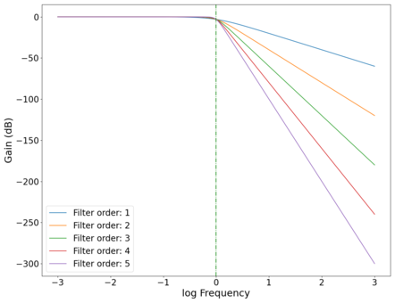 Plot of the (power) gain Failed to parse (SVG (MathML can be enabled via browser plugin): Invalid response ("Math extension cannot connect to Restbase.") from server "https://wikimedia.org/api/rest_v1/":): {\displaystyle G(f)} vs log frequency Failed to parse (SVG (MathML can be enabled via browser plugin): Invalid response ("Math extension cannot connect to Restbase.") from server "https://wikimedia.org/api/rest_v1/":): {\displaystyle \log_{10}f} of low-pass Butterworth filters of different orders with cutoff frequency Failed to parse (SVG (MathML can be enabled via browser plugin): Invalid response ("Math extension cannot connect to Restbase.") from server "https://wikimedia.org/api/rest_v1/":): {\displaystyle f=1} Hz, showing the increasing rate of frequency rejection as the order of the filters increase. Green dotted line marks cutoff frequency Failed to parse (SVG (MathML can be enabled via browser plugin): Invalid response ("Math extension cannot connect to Restbase.") from server "https://wikimedia.org/api/rest_v1/":): {\displaystyle f_c = 1} Hz.
 -
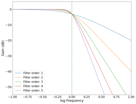 Plot of the gain Failed to parse (SVG (MathML can be enabled via browser plugin): Invalid response ("Math extension cannot connect to Restbase.") from server "https://wikimedia.org/api/rest_v1/":): {\displaystyle G(f)} vs log frequency Failed to parse (SVG (MathML can be enabled via browser plugin): Invalid response ("Math extension cannot connect to Restbase.") from server "https://wikimedia.org/api/rest_v1/":): {\displaystyle \log_{10}f} of different order low-pass Butterworth filters with the cutoff point magnified, showing increasing sharpness in the cutoff behaviour as the order of the filters increase. Green dotted line marks cutoff frequency Hz.
 -
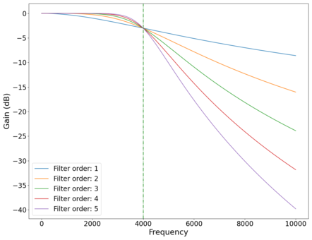 Plot of the Failed to parse (SVG (MathML can be enabled via browser plugin): Invalid response ("Math extension cannot connect to Restbase.") from server "https://wikimedia.org/api/rest_v1/":): {\displaystyle G(f)} vs frequency Failed to parse (SVG (MathML can be enabled via browser plugin): Invalid response ("Math extension cannot connect to Restbase.") from server "https://wikimedia.org/api/rest_v1/":): {\displaystyle f} of different order low-pass Butterworth filters. Green dotted line marks cutoff frequency Failed to parse (SVG (MathML can be enabled via browser plugin): Invalid response ("Math extension cannot connect to Restbase.") from server "https://wikimedia.org/api/rest_v1/":): {\displaystyle f_c = 4000} Hz.
 -
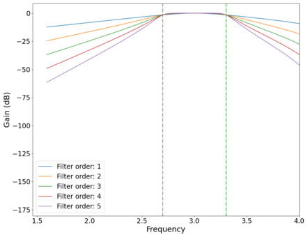 Plot of the Failed to parse (SVG (MathML can be enabled via browser plugin): Invalid response ("Math extension cannot connect to Restbase.") from server "https://wikimedia.org/api/rest_v1/":): {\displaystyle G(f)} vs log frequency Failed to parse (SVG (MathML can be enabled via browser plugin): Invalid response ("Math extension cannot connect to Restbase.") from server "https://wikimedia.org/api/rest_v1/":): {\displaystyle \log_{10}f} of different order band-pass Butterworth filters. Green dotted lines mark cutoff frequencies at Failed to parse (SVG (MathML can be enabled via browser plugin): Invalid response ("Math extension cannot connect to Restbase.") from server "https://wikimedia.org/api/rest_v1/":): {\displaystyle 100} and Failed to parse (SVG (MathML can be enabled via browser plugin): Invalid response ("Math extension cannot connect to Restbase.") from server "https://wikimedia.org/api/rest_v1/":): {\displaystyle 2000} Hz.


The Butterworth filters in this work will be created using the signal package from the SciPy Python library. The butter function generates a Butterworth filter that can be specified to be low-pass, high-pass, or band-pass. An example of a band-pass filter implemented programmatically is shown above. We see slight distortions (non-zero curvature in the roll-off limit vs flat in an ideal filter) at higher frequencies due to the Nyquist frequency of the digital filter, which is a consequence of the Nyquist–Shannon sampling theorem.
An example of a band-pass 2nd order Butterworth filter implemented on white noise is seen in the image below.

An audio comparison between the unfiltered and filtered waves can be found here: White noise and Filtered noise.
Concept

In this experiment, we attempt to convert an impinging light source into a voltage signal that reproduces an audio signal using a photodiode. The idea behind this is inspired by the concept of amplitude modulation (AM) in electronic communication. In AM, a signal (information) wave is transmitted via a carrier wave with a frequency much greater than the frequency range of the signal wave, and the receiver locks on to the frequency Failed to parse (SVG (MathML can be enabled via browser plugin): Invalid response ("Math extension cannot connect to Restbase.") from server "https://wikimedia.org/api/rest_v1/":): {\displaystyle f_c} .

The amplitude of the carrier wave is modulated by the amplitude of the signal, meaning the envelope of the transmitted wave contains the signal information. The receiver then reconstructs the signal by measuring the envelope of the received wave. An example of the three waves described is shown in the animation on the right.
In this project, a laser is reflected off a mirror attached to a surface and onto a photodiode, generating a measurable voltage. When the surface vibrates, the deflection of the mirror causes the laser to move off the photodiode, reducing the voltage to zero. Since the laser has a non-zero spot size and can be approximated to have a Gaussian profile (in the TEM00 mode), intermediate levels of modulation other than 1 or 0 can also be obtained for small enough deflections.
In analogy with the amplitude modulation described above, the laser functions as a carrier wave which the photodiode is sensitive to, and the signal wave is the sound wave that causes the surface to vibrate, modulating the amplitude of the laser that reaches the photodiode. In theory, this should allow us to reconstruct the signal wave by directly converting the voltage measured into a sound wave.
The voltage measured should correspond almost directly to the envelope of the carrier wave if we use a visible light laser. This is because the frequency of visible light is in the hundreds of THz (~Failed to parse (SVG (MathML can be enabled via browser plugin): Invalid response ("Math extension cannot connect to Restbase.") from server "https://wikimedia.org/api/rest_v1/":): {\displaystyle 10^{14}} to Failed to parse (SVG (MathML can be enabled via browser plugin): Invalid response ("Math extension cannot connect to Restbase.") from server "https://wikimedia.org/api/rest_v1/":): {\displaystyle 10^{15}} Hz), while the cutoff frequency of the photodiode used[4] is on the order of Failed to parse (SVG (MathML can be enabled via browser plugin): Invalid response ("Math extension cannot connect to Restbase.") from server "https://wikimedia.org/api/rest_v1/":): {\displaystyle 10^7} Hz. As such, the high frequency component of the carrier wave (laser) is effectively filtered out by the photodiode acting as a low-pass filter, leaving just the lower frequency amplitude modulation component in an ideal case.
Quality of Reproduced Audio
On top of just judging how close the reproduced audio is to the original audio by listening to it, we can use a second measure to objectively quantify the quality or "closeness" of the reproduced audio to the original. The musicg module was used, which contained a fingerprint package that allows the "fingerprinting" of audio files by obtaining the spectrogram at each sample interval. The same module also allows for the comparison of the fingerprints of both files, giving a similarity score Failed to parse (SVG (MathML can be enabled via browser plugin): Invalid response ("Math extension cannot connect to Restbase.") from server "https://wikimedia.org/api/rest_v1/":): {\displaystyle S_0}
. The code for calculating similarity works as follows:
- The audio files are split into "frames" based on the sample rate,
- the spectrogram of each frame is calculated,
- the files are "aligned" based on the alignment with the maximum "match" count between the two files,
- the total number of matches is divided by the total number of frames to give a similarity score showing the number of matches per frame.
The value of a "match" is calculated by the difference between the spectrograms in each frame, the more the spectrograms overlap, the greater the value of a match. The raw value of the similarity score is in arbitrary units that is consistent across different pairs of audio compared. In this project, we will treat a score of 1.0 (at least one "match" per frame) and above to be a perfect reproduction of the audio. Any score less than 1.0 represents a less than perfect reproduction of the audio. Because the code only looks for matches (score does not get deducted by lack of a match), this is a good way to quantify reproduction quality with small amounts of background noise being acceptable.
The table below shows an example of the similarity score between 3 different audio files.
| Failed to parse (SVG (MathML can be enabled via browser plugin): Invalid response ("Math extension cannot connect to Restbase.") from server "https://wikimedia.org/api/rest_v1/":): {\displaystyle S_0} | Pure 200 Hz tone | Pure 200 Hz tone + white noise | Pure 300 Hz tone | Pure 300 Hz tone + white noise |
|---|---|---|---|---|
| Pure 200 Hz tone | 3.35714 | - | - | - |
| Pure 200 Hz tone + white noise | 0.63265 | 2.92857 | - | - |
| Pure 300 Hz tone | 0.0 | 0.0 | 3.35714 | - |
| Pure 300 Hz tone + white noise | 0.02041 | 0.01020 | 0.67347 | 3.06122 |
Difficulties
Even though the module provided a way to quantify the similarity between two pieces of audio (something that is not trivial to do), we had to make some modifications to the source code. Due to the module being written for a depreciated version of Java from over a decade ago, it relies on libraries that are no longer supported. As such, we had to reimplement a small portion of the Fast Fourier Transform algorithm within the source code, which took quite some time (as we are trained in Python, not Java!). After quite a bit of relearning Java, we managed to get the module and the functions required working.
We found that with large levels of distortion and noise, this metric becomes significantly less useful as it cannot account for frequency shifts and large shifts in the dynamics of the audio. An example for the former would be two tracks that are slightly pitch shifted relative to each other which would be trivial for a human to indicate a high similarity score for, but this method will give a low similarity score for. An example of the latter would be a track with the volume of the low frequencies boosted significantly, which again would still keep a high similarity score when judged by a human, but will be poorly judged by this method as the code normalises the spectrograms before conducting the similarity check (causing some features to "disappear" if other features get too loud). This second effect will primarily be caused by resonance as we will observe later. We will see later on that other than for simple pure frequency comparisons, this metric is not a very good indicator of similarity due to the large amounts of distortion our setup introduces. The similarity scores will still be indicated, but the score will be coloured red to indicate that we do not think it is a reliable measure of similarity.
For future reference, a similarity metric that uses something like computer vision to match features in the spectrograms or deep learning to identify spectrogram features might be more useful.
Original Setup

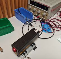
The original setup was created with as few components as possible to create a baseline performance that we can compare to. A schematic of the setup is shown in the image above. A Melles Griot HeNe laser with a wavelength of 632.8 nm was used to function as the carrier wave. The laser impinges upon a mirror attached to a surface near a pair of speakers, then gets reflected onto a photodiode which is connected to an oscilloscope. The setup is aligned such that when the surface vibrates along with the mirror, an angular displacement of the laser beam occurs and there is a longitudinal displacement of the laser spot at the photodiode. The mirror and photodiode are separated by about 6 metres, so any small angular displacement results in a large longitudinal displacement and resulting shift in total power incident on the photodiode, changing the voltage output detected by the oscilloscope. This setup implements the amplitude modulation discussed previously by converting small physical motions to changes in the amplitude of the voltage recorded. The components are shown below.
-
 Laser connected to power supply.
 -
 Mirror mounted on original surface constructed with a balloon stretched over a 3D printed cylinder.
 -
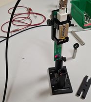 Laser spot on photodiode after reflection off the mirror.
 -
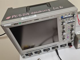 Oscilloscope used to measure the signal from the photodiode.


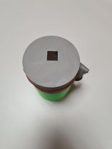
Note that as seen in the photo of the photodiode, the laser is not centered on the photodiode but instead on one corner. We found that this improved the signal received, as this allowed small deflections to also be detected when the laser shifted in any direction, including towards the center of the photodiode (which increased the overall power on the photodiode). In contrast, if the laser is centered on the photodiode, small deflections will not be detected as the voltage output by the photodiode is only dependent on the total power received and not the location on its surface.
Oscilloscope Settings
The following settings were used for the oscilloscope:
- 1 MΩ input impedance
- 0.1 mV voltage resolution
- 50 μs time resolution
The choice of the time resolution was done as a compromise between the Nyquist frequency placing a lower bound on the number of samples per second we can take, and wanting a reasonably long recording placing an upper bound on the number of samples per second (since the oscilloscope has a limited amount of memory to store recordings). Our current choice of 20 kilosamples per second gives a Nyquist frequency of 10 kHz, which should capture a decent frequency range for low quality recordings. This also gives us a 5 second long recording, which we decided was the minimum recording length which we can demonstrate the ability of our setup with.
Results (Original Setup)
Pure Frequencies
We tested the original setup with pure tones as a proof of concept in order to determine if such a setup can transmit any information. The spectra of the different tones tested along with the audio reconstructed from the output of the receiver are seen in the table below. The red lines in each graph show the frequency of the test tone played. From the spectra and audio, it is clear that the concept works, and we are able to transmit audio information simply by reflecting a laser off a surface near the audio, and collecting the reflected beam with a photodiode, followed by recording the voltage output from the photodiode. A second order low-pass Butterworth filter was applied to each audio recording at 2000 Hz in order to remove the background noise.
Even though we played pure frequencies, we see multiple spikes at integer multiples of those frequencies, indicating that the harmonics are also induced on the surface, which is expected and is a characteristic of the surface, also known as timbre in music. The average difference between the frequency in the reconstructed audio and the frequency transmitted Failed to parse (SVG (MathML can be enabled via browser plugin): Invalid response ("Math extension cannot connect to Restbase.") from server "https://wikimedia.org/api/rest_v1/":): {\displaystyle \Delta f_0} is also indicated in the table, showing small deviations between the reconstructed signal and the transmitted signal.
We note that for some frequencies (300 Hz, 500 Hz), the audio obtained is not correct. This is because a higher harmonic was activated more strongly than the fundamental for those frequencies, causing the harmonics to be recorded instead. For 600 Hz and 700 Hz, barely any signal could be heard which is a function of both the weaker response of the vibrating surface to those frequencies, and our perception of volume being different for different frequencies.
| Transmitted Frequency | vs Failed to parse (SVG (MathML can be enabled via browser plugin): Invalid response ("Math extension cannot connect to Restbase.") from server "https://wikimedia.org/api/rest_v1/":): {\displaystyle \log_{10}{f}} | Failed to parse (SVG (MathML can be enabled via browser plugin): Invalid response ("Math extension cannot connect to Restbase.") from server "https://wikimedia.org/api/rest_v1/":): {\displaystyle P} vs Failed to parse (SVG (MathML can be enabled via browser plugin): Invalid response ("Math extension cannot connect to Restbase.") from server "https://wikimedia.org/api/rest_v1/":): {\displaystyle f} | Failed to parse (SVG (MathML can be enabled via browser plugin): Invalid response ("Math extension cannot connect to Restbase.") from server "https://wikimedia.org/api/rest_v1/":): {\displaystyle P} vs Failed to parse (SVG (MathML can be enabled via browser plugin): Invalid response ("Math extension cannot connect to Restbase.") from server "https://wikimedia.org/api/rest_v1/":): {\displaystyle \log_{10}{f}} (Filtered) | Failed to parse (SVG (MathML can be enabled via browser plugin): Invalid response ("Math extension cannot connect to Restbase.") from server "https://wikimedia.org/api/rest_v1/":): {\displaystyle \Delta f_0} / Hz | Audio | Failed to parse (SVG (MathML can be enabled via browser plugin): Invalid response ("Math extension cannot connect to Restbase.") from server "https://wikimedia.org/api/rest_v1/":): {\displaystyle S_0} (source vs unfiltered) | Failed to parse (SVG (MathML can be enabled via browser plugin): Invalid response ("Math extension cannot connect to Restbase.") from server "https://wikimedia.org/api/rest_v1/":): {\displaystyle S_0} (source vs filtered) |
|---|---|---|---|---|---|---|---|
| 100 | 
|

|

|
-0.04 0.13 | Unfiltered vs filtered | 0.09184 | 0.15306 |
| 200 | 
|

|

|
0.8 Failed to parse (SVG (MathML can be enabled via browser plugin): Invalid response ("Math extension cannot connect to Restbase.") from server "https://wikimedia.org/api/rest_v1/":): {\displaystyle \pm} 2.3 | Unfiltered vs filtered | 0.64286 | 0.5 |
| 300 | 
|

|

|
0.08 Failed to parse (SVG (MathML can be enabled via browser plugin): Invalid response ("Math extension cannot connect to Restbase.") from server "https://wikimedia.org/api/rest_v1/":): {\displaystyle \pm} 0.14 | Unfiltered vs filtered | 0.0 | 0.0 |
| 400 | 
|

|

|
0.32 Failed to parse (SVG (MathML can be enabled via browser plugin): Invalid response ("Math extension cannot connect to Restbase.") from server "https://wikimedia.org/api/rest_v1/":): {\displaystyle \pm} 0.28 | Unfiltered vs filtered | 0.22449 | 0.18367 |
| 500 | 
|

|

|
-0.07 Failed to parse (SVG (MathML can be enabled via browser plugin): Invalid response ("Math extension cannot connect to Restbase.") from server "https://wikimedia.org/api/rest_v1/":): {\displaystyle \pm} 0.15 | Unfiltered vs filtered | 0.60204 | 0.66327 |
| 600 | 
|

|

|
1.6 Failed to parse (SVG (MathML can be enabled via browser plugin): Invalid response ("Math extension cannot connect to Restbase.") from server "https://wikimedia.org/api/rest_v1/":): {\displaystyle \pm} 3.6 | Unfiltered vs filtered | 0.02040 | 0.19388 |
| 700 | 
|

|

|
0.07 Failed to parse (SVG (MathML can be enabled via browser plugin): Invalid response ("Math extension cannot connect to Restbase.") from server "https://wikimedia.org/api/rest_v1/":): {\displaystyle \pm} 0.14 | Unfiltered vs filtered | 0.56122 | 0.68367 |


Real-World Audio
After testing the pure frequencies, we tested out two clips from a person speaking. We found that due to the response of our stretched balloon membrane being highly focused around the vibrational modes of the membrane, the transmitted signal is extremely distorted. Furthermore, we observed the phenomenon of clipping when certain frequencies cause large amplitude vibrations in the membrane. As the photodiode has a minimum voltage output when the laser spot is completely off the photodiode corresponding to a certain vibrational amplitude, there is a limit to the vibrational amplitude it can capture, meaning any vibration above that amplitude gets flattened to that level. These "clipped" sections are not only much louder than the surrounding sections, they introduce huge amounts of distortion in the reconstructed audio as the clipped section approaches a square wave, introducing high frequency components not present in the original audio.
Seashells
The first piece of audio used was a classic tongue twister found here. The images below show the raw voltage over time recorded, showing large audio clipping and transient asymmetry. After passing the audio through a 2nd order band-pass Butterworth filter with the passband from 100 Hz to 2000 Hz, the waveform looks significantly more like what we would expect from a normal audio waveform. This is because the asymmetry in the transient spikes correspond to high frequency components that are removed during the filtering. The recorded audio can be found here (unfiltered) and here (filtered) (volume warning due to clipping).
-
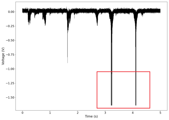 Voltage recorded from the photodiode (mean subtracted) vs time showing transient spikes and clipping (in red).
 -
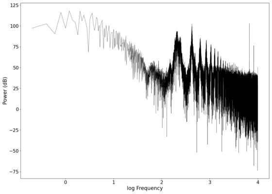 Log-log spectrum of the unfiltered recording.
 -
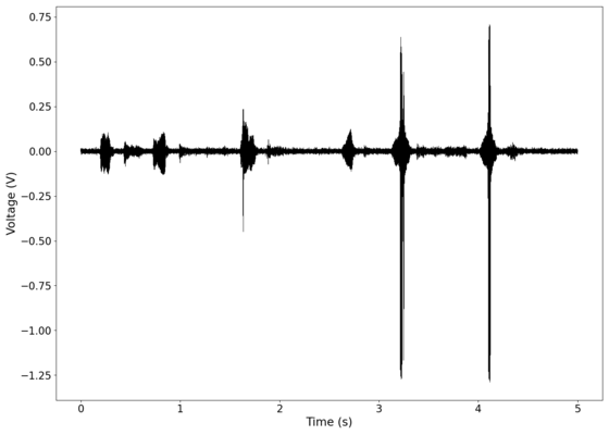 Original signal after band-pass filtering showing significantly less asymmetry.
 -
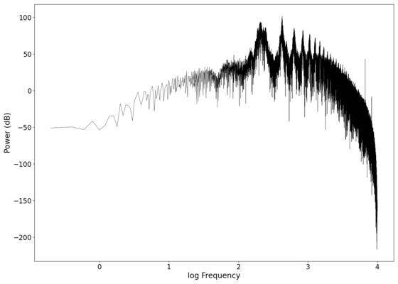 Log-log spectrum of the filtered recording.


The similarity scores are shown in the table below.
| Failed to parse (SVG (MathML can be enabled via browser plugin): Invalid response ("Math extension cannot connect to Restbase.") from server "https://wikimedia.org/api/rest_v1/":): {\displaystyle S_0} | Source | Unfiltered | Filtered |
|---|---|---|---|
| Source | 2.94444 | - | - |
| Unfiltered | 0.03061 | 3.25510 | - |
| Filtered | 0.04082 | 0.21429 | 2.95918 |
Bread
The second piece of audio used was another tongue twister found here. The images below show the same as in those in the previous section, albeit with significantly less clipping. The recorded audio can be found here (unfiltered) and here (filtered).
-
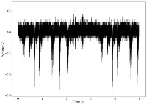 Voltage recorded from the photodiode (mean subtracted) vs time showing transient spikes.
 -
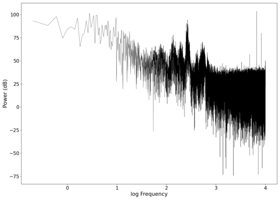 Log-log spectrum of the unfiltered recording.
 -
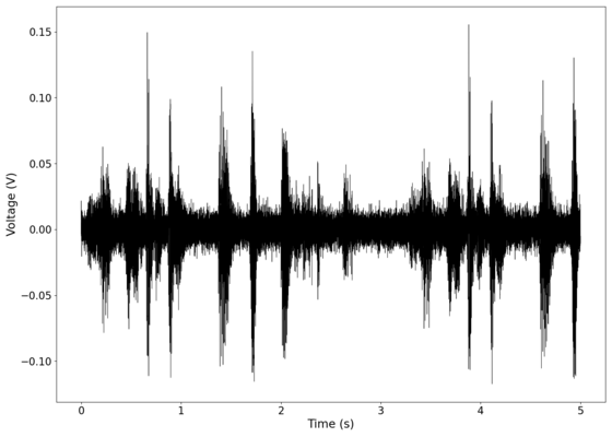 Original signal after band-pass filtering showing significantly less asymmetry.
 -
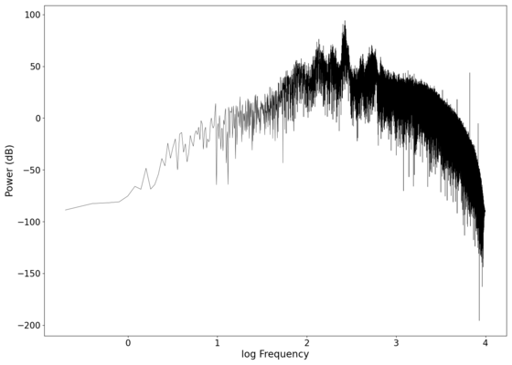 Log-log spectrum of the filtered recording.


The similarity scores are shown in the table below.
| Failed to parse (SVG (MathML can be enabled via browser plugin): Invalid response ("Math extension cannot connect to Restbase.") from server "https://wikimedia.org/api/rest_v1/":): {\displaystyle S_0} | Source | Unfiltered | Filtered |
|---|---|---|---|
| Source | 2.98477 | - | - |
| Unfiltered | 0.02041 | 3.11224 | - |
| Filtered | 0.01020 | 0.02041 | 2.89796 |
Discussion
Even through the distortion and information lost due to the response of the vibrating surface, one is able to tell that this audio matches the transmitted audio when directly comparing them. While we would already classify this as a success based on our original objectives, we wondered if it was possible to make small and easy modifications to our setup to improve on the quality of the transmission. We identified two main problems:
- The response of the balloon membrane used was too sharp and centered around its vibrational modes, causing either large amounts of clipping if we wanted to capture the audio in the frequencies with a smaller response, or only capturing the frequencies near the vibrational modes of the surface.
- The large laser spot and large photosensitive area of the photodiode ironically work together to make the setup insensitive to small movements in the laser spot. For a wide range of movement in a wide range of directions, the overall power incident on the photodiode stays roughly the same as the photodiode simply captures different sections (that add up to about the same overall power) of the laser spot.
With these problems in mind, we found two relatively simple fixes (that can even be implemented with common household items!) that we will discuss in the next section.
Modified Setup

We made two main modifications to our setup that led to large improvements in the quality of the recordings based on some heuristics that we observed.
Firstly, we added an aperture in front of the photodiode to improve the sensitivity of the setup to small deviations in the laser spot location as the spot only has to move a small distance before being completely blocked by the aperture. The circular aperture also makes sensitivity of the setup isotropic relative to the direction of movement of the laser spot (as opposed to the original setup, where the response is expected to be anisotropic since the total power impinging on the photodiode depends on the direction the laser spot gets deflected in). With the small pinhole only sampling a small area within the laser spot, this should also theoretically improve the sensitivity to very small movements which cause the pinhole to sample different regions within the laser spot which has (approximately) a Gaussian distribution, causing a different amount of incident power on the photodiode. The aperture also blocked most of the stray laser light caused by diffraction of the initial spot, which would add noise to the recordings. The aperture is seen included within the setup in the image on the right. Note that this can easily be replicated with common items like a pinhole in a cardboard box, we just used the aperture because it was available in the lab.

Secondly, we replaced the surface the mirror was mounted on with a cardboard box, as we noticed that the stretched rubber balloon had a very strong response within its resonant modes. To a first order approximation, we treat the surfaces as simply supported plates. The spacings of the modes are proportional to the square root of the elastic modulus of the material, inversely proportional to the square root of the areal density, and inversely proportional to the square of the area[5]. As a result, we expect the new surface (which has a lower elastic modulus, larger areal density, and much larger surface area) to have closer spaced modes, which would broaden the frequency response of the surface and hopefully avoid the sharp spikes in audio at specific frequencies. The larger surface also has the added benefit of capturing a larger portion of the audio power output by the speakers, leading to more efficient conversion of the audio power to signal power.
A schematic of the new setup is seen below.

Results (Modified Setup)
Background Noise

To characterise the noise present in the system, we took multiple measurements of the system with the setup shown on the right, with the aperture closed to a pinhole. Note that the laser spot on the photodiode appears larger in the photo than in reality, with most of the "spot" in the photo being camera bloom from the bright spot.
The measurement was done with the laser on as the output of the laser has been observed to drift over time, and will contribute to the noise in the system. The images below show the three measurements we did, followed by an average of the three readings. The results that we obtained for the background noise of the system are remarkably similar to the noise profile of other electrical systems[6], showing noise with a corner frequency of ~Failed to parse (SVG (MathML can be enabled via browser plugin): Invalid response ("Math extension cannot connect to Restbase.") from server "https://wikimedia.org/api/rest_v1/":): {\displaystyle 100} Hz, and white noise above that. We hypothesise that the portion with the white noise comes from a combination of ambient light in the room, shot noise, and Johnson-Nyquist noise. Due to the solid state devices present in our system, it is likely that the Failed to parse (SVG (MathML can be enabled via browser plugin): Invalid response ("Math extension cannot connect to Restbase.") from server "https://wikimedia.org/api/rest_v1/":): {\displaystyle 1/f} noise arises from a combination of flicker noise in all the electrical components and generation-recombination noise in the laser gain medium and photodiode.

-
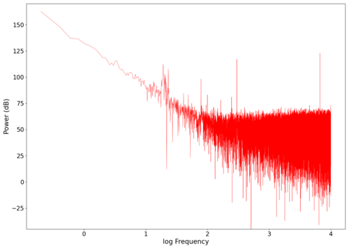 Spectrum of background noise (first reading). Audio can be found here.
 -
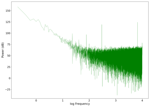 Spectrum of background noise (second reading). Audio can be found here.
 -
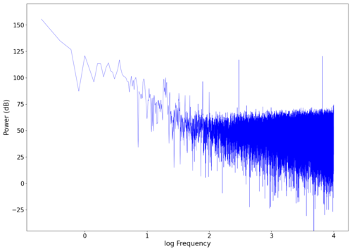 Spectrum of background noise (third reading). Audio can be found here.
 -
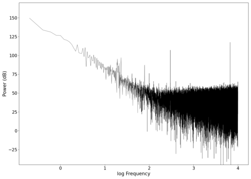 Spectrum of background noise (averaged). Audio can be found here.


Pure Frequency
We again played a test tone of 200 Hz with our new setup to look at the spectral response of our system. The spectral plot is shown below, and unfortunately, the new cardboard box surface appears to have introduced more distortion in the very low frequencies (<100 Hz). We did not test this, but we hypothesise that the larger box being weighed down onto the table (which is not vibration isolated) caused the entire box-speaker-table system to be coupled which caused strange resonant behaviour in the frequencies below the driving frequency. This is justified by there being less energy in the frequencies that are a rational fraction of the driving frequency, suggesting that the entire system is acting as a coupled oscillator and the table is possibly taking energy away from those frequencies. The reason we did not test this hypothesis is that the additional resonant behaviour at low frequencies can easily be filtered out with a band-pass filter, and we chose not to dedicate more time to investigating this (as we only had ~8 weeks to complete this experiment during the semester). We can see from the graph of the filtered signal below that the band-pass filter almost completely eliminates this problem.
-
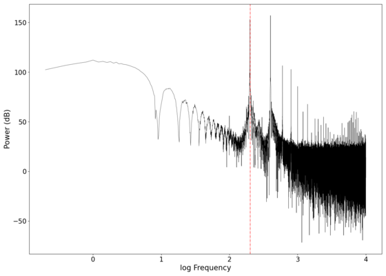 Power vs log frequency plot of the received signal for a transmitted signal of 200 Hz (red dotted line).
 -
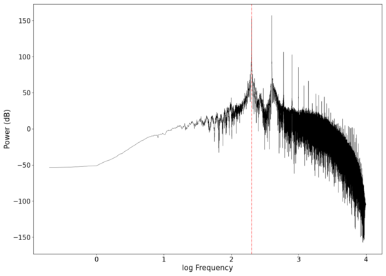 Power vs log frequency plot of the filtered signal.


Despite the added distortion mentioned previously over our original setup, we stuck with this modified setup for two main reasons.
- The new surface greatly increased the amount of power captured from the speakers as expected. This, along with the increased sensitivity the added aperture provides, greatly increased the strength of the signal at the receiving end. Comparing the filtered audio from the original surface to the new surface, we note a marked improvement in audio quality as the old setup produced a signal that was barely above the noise floor and needed digital gain to be added, while the new setup produced such a strong and clear signal that we reduced the signal by a factor of 10 in order to have audio that is not too loud.
- The new surface has a response curve that is significantly "flatter" than the old balloon membrane, with the differences in their spectral response shown below.
-
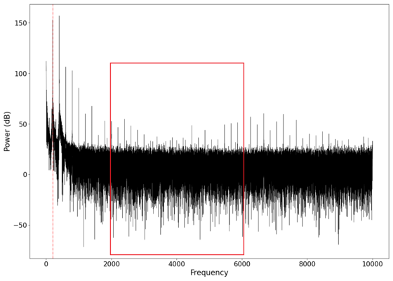 Spectral response of the new surface, showing a relatively "flat" overall response especially in the marked region when compared to the old surface.
 -
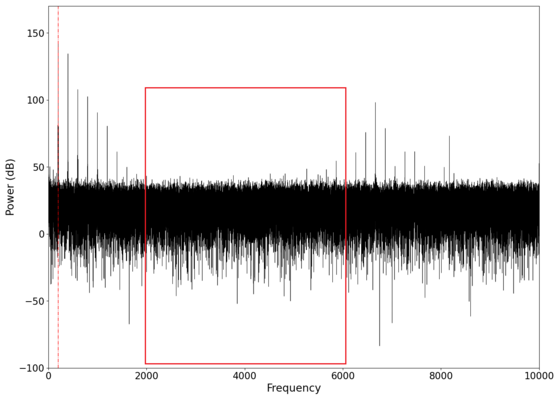 Spectral response of the old surface, showing a significantly less flat response with almost no response in the marked region.


Real-World Audio
The modified setup managed to record significantly higher fidelity audio. We tested a wide range of types of audio including speech and music, and the best pieces of audio will be shown here. The rest of the audio files generated can be found at this GitHub page. Additionally, due to a mix of samples not being locally available (found online) and the difficulties mentioned in the Quality of Reproduced Audio section, the similarity scores will no longer be reported here (random testing found that the score was quite arbitrary, two samples that are auditorily very similar to the human ear can have seemingly random similarity scores).
Along with the original 2nd order band-pass Butterworth filter with the pass-band from 100 Hz to 2000 Hz, an additional 1st order band-pass Butterworth filter with the pass-band from 900 Hz to 2000 Hz was applied after, followed by artificial digital gain. These values were manually picked and were found to produce the best (most recognisable) audio. The second filtering step introduces some additional noise due to ringing artifacts caused by the Gibbs phenomenon, which then gets boosted to form a more "noisy" background. The low frequency audio also decreases in quality after the second filtering step. However, we found that for most of the audio that we tested, those sacrifices partly corrected for the bass-heavy response curve of our setup, allowing the final piece of audio to be more recognisable across all frequencies. This second filtering step can be seen as a manually tuned equaliser specific to our setup, and can of course be left unused if the audio is low frequency audio.
Due to the ringing artifacts mentioned previously, we intentionally used a "gentle" method for equalising with the lowest order filter we had. Our initial tests with "harsh" equalising where we altered the gain sharply resulted in very strong echoing and ringing (as expected). The ringing artifacts can be heard clearly in our samples here: Original and Naive Equalising.
Seashells
As a first test of our new setup, we play the same tongue twister in the seashells section found here. The graphs of the recorded signal in both the frequency and time domains can be seen below.
-
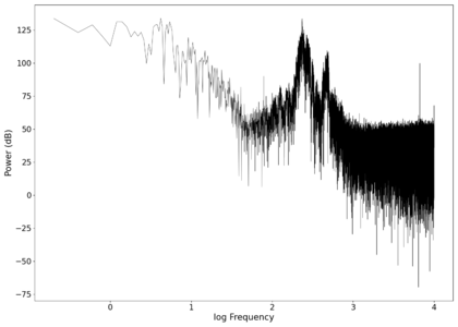 Spectrum of the unfiltered audio.
 -
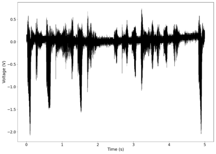 Raw voltage vs time recorded (with mean subtracted).


-
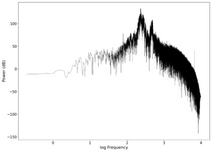 Spectrum of the filtered audio (first filter to remove background noise).
 -
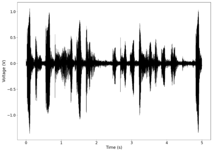 Voltage vs time after first filter applied.


-
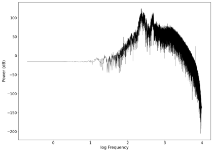 Spectrum of the filtered audio (with manual equaliser applied).
 -
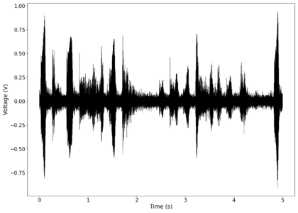 Voltage vs time after equaliser applied.


We can see the effect the second filtering step has, which is to "flatten" the volume of the audio from about 100 Hz to 1500 Hz. While it is not the best action to perform if we want to preserve quality and dynamic range, our goal is to have recognisable audio and a flat spectral response in the kHz range usually accounts for most of that[7].
The reconstructed audio tracks can be heard here: Unfiltered, filtered, filtered and equalised. While the quality is not perfect, there is a huge improvement in terms of recognisability and intelligibility across the low to mid frequency ranges. Compared to the original setup, the words are intelligible with only the fricative sounds missing. This is evidence that our small modifications to the original setup worked.
Curb Your Enthusiasm
The second piece of audio tested was the start of the popular theme song from Curb Your Enthusiasm. The graphs of the recorded signal in both the frequency and time domains can be seen below.
-
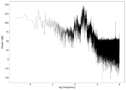 Spectrum of the unfiltered audio.
 -
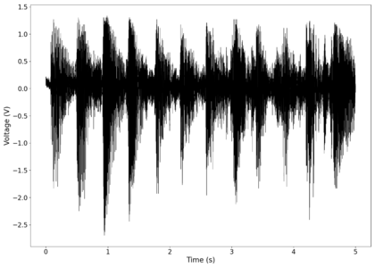 Raw voltage vs time recorded (with mean subtracted).


-
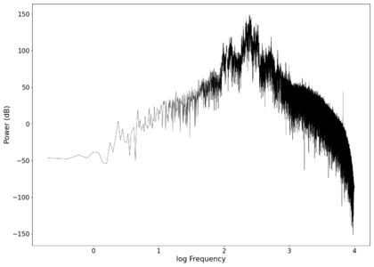 Spectrum of the filtered audio (first filter to remove background noise).
 -
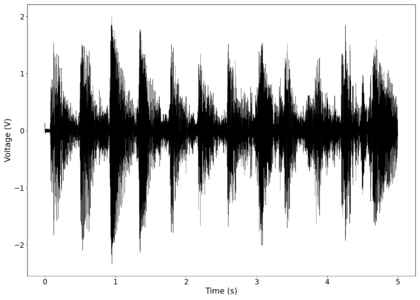 Voltage vs time after first filter applied.


-
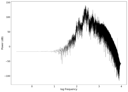 Spectrum of the filtered audio (with manual equaliser applied).
 -
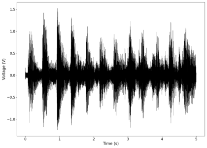 Voltage vs time after equaliser applied.


The reconstructed audio tracks can be heard here: Unfiltered, filtered, filtered and equalised. Again, the audio is pretty good and captures most of the fundamental portions of the transmitted audio with only slight distortion and noise added, so the reconstructed audio is still recognisably the same as the original.
Nocturne
Another piece of audio that we tested is the start of Nocturne, Op. 9, No. 2, found here. The graphs of the recorded signal in both the frequency and time domains can be seen below.
-
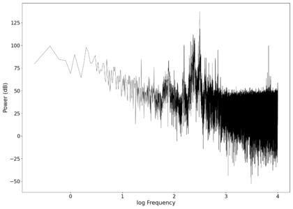 Spectrum of the unfiltered audio.
 -
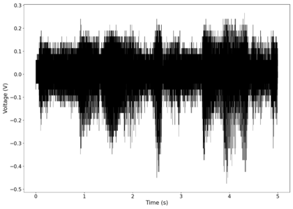 Raw voltage vs time recorded (with mean subtracted).


-
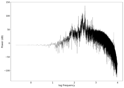 Spectrum of the filtered audio (first filter to remove background noise).
 -
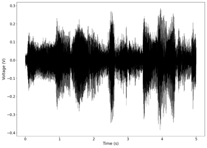 Voltage vs time after first filter applied.


-
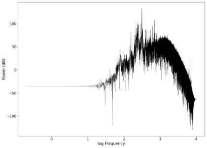 Spectrum of the filtered audio (with manual equaliser applied).
 -
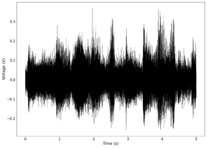 Voltage vs time after equaliser applied.


The reconstructed audio tracks can be heard here: Unfiltered, filtered, filtered and equalised. The equalising step did not help much for this as most of the original audio was already within a relatively flat section of the spectrum.
Lesson Audio
We tested lesson audio from the Recorded sessions, specifically session 2. This test was to determine how audio that was initially recorded in less than ideal settings (a lecture theatre) would perform. We took samples from different sections in the recording, and the processed recordings can be found in the table below.
| Samples | |||
|---|---|---|---|
| 1 | Unfiltered | Filtered | Filtered and Equalised |
| 2 | Unfiltered | Filtered | Filtered and Equalised |
| 3 | Unfiltered | Filtered | Filtered and Equalised |
| 4 | Unfiltered | Filtered | Filtered and Equalised |
Due to the audio already being slightly muffled in the source, the words are not as intelligible as the other example in the seashells section. However, the cadence and tone of our professor still distinctly carries through into the reproduced audio and is recognisable.
Impact of the Aperture
We made two changes to our original setup to get this modified setup: The change in the vibrating surface, and the addition of a pinhole aperture. We can see the improved response of the new surface in the graphs above which directly translates to the improved quality of the reconstructed audio. However, our claim that the aperture improves the sensitivity of the setup was not proven as we attributed the increased sensitivity to both the aperture and the new surface collecting much more audio energy. To decouple these two effects, we performed a test with and without the aperture with the new surface.
We decided to use cello music from Bach which contains a lot of energy in the low frequencies (which our surface is most sensitive to) in order to maximise the deflection in the setup without the aperture (and give it the highest chance of detecting a signal). We only apply the first filter in this section to filter out the background noise as we are just testing the sensitivity and hence just looking for the strength of the signal without equalising. In the time series graphs below, we see a clear signal in the setup with the aperture, while the setup without the aperture appears to just contain noise. This is made clear with the reconstructed audio with the aperture and without the aperture. Without the aperture, the setup is not sensitive enough and any signal is well below the noise floor of the system. With the aperture, the transmitted signal is significantly above the noise floor and is very recognisable.
-
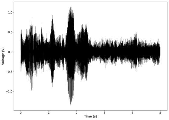 Voltage vs time of signal after filtering out background noise in the setup with aperture included.
 -
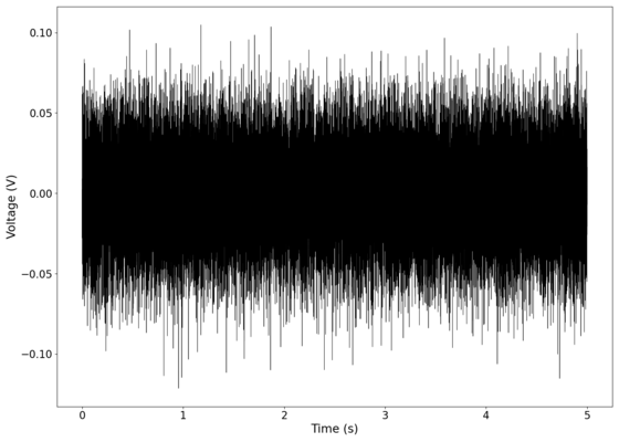 Voltage vs time of signal after filtering out background noise in the setup with aperture excluded.


Discussion
We were able to achieve our initial objectives of transmitting audio information with a laser reflecting off a surface near the audio source. The quality and intelligibility of the audio along with the sensitivity of the setup was then greatly improved by making two relatively small modifications to our setup. What is noteworthy was that other than the oscilloscope (which we used to visually monitor the sound but could have replaced with a much cheaper sound card that records the signal from the photodiode), every other component can be found lying around the house or bought extremely cheaply. We intentionally chose to not use specialised equipment that can only be found in a lab in order to determine if this can be achieved with cheap off-the-shelf components and some small custom modifications, and our results above show that this is possible.
However, we have some suggestions for anyone attempting this in the future that we expect will greatly improve the results with relatively little effort/cheap materials.
- Vibrationally isolate the vibrating surface from the table to some degree, this can be done with some cheap rubber padding. We suspect that the coupling of the surface to the table introduced some distortion, but did not have the time to test it.
- Add a hardware amplifier between the photodiode and oscilloscope. While our setup was already sensitive enough to produce a signal well above the noise floor of the system, a hardware amplifier would further raise the level of the signal which could give the setup more "wiggle room" to perform digital processing on.The amount of quality that our digital processing steps could add to the audio was limited by this.
- Use third-party software like Audacity to do the digital signal processing as the algorithms present in those software are significantly more mature and allow for a lot more fine-tuning. We opted not to do this in our project as we wanted to know the specifics of our digital signal processing steps (which are unclear in the black box algorithms in Audacity), but if that is not an issue for someone doing this in the future, the third-party algorithms are likely to result in higher quality reconstructions.
References
- ↑ "Generational Wi-Fi® User Guide". www.wi-fi.org. October 2018.
- ↑ Bluetooth Core Specification Version 5.3 Feature Enhancements. www.bluetooth.com. June 2021.
- ↑ S. Butterworth, "On the Theory of Filter Amplifiers," Experimental Wireless and the Wireless Engineer, Vol. 7, 1930, pp. 536-541
- ↑ Hamamatsu Photonics. Datasheet for S5980/S5981/S5870 series Si PIN photodiodes Jan 2021
- ↑ Irvine, T. (2019) An Introduction to Shock and Vibration Response Spectra.
- ↑ Kiely, R. (2017) Understanding and Eliminating 1/f Noise. Analog Dialogue 51-05, May 2017
- ↑ Monson, B., Hunter, E., Lotto, A. and Story, B. (2014) The perceptual significance of high-frequency energy in the human voice. Front. Psychol., Vol. 5, [1]