Homodyne detection: Difference between revisions
Xie Chengkun (talk | contribs) |
Johnkhootf (talk | contribs) No edit summary |
||
| (10 intermediate revisions by the same user not shown) | |||
| Line 37: | Line 37: | ||
[[Image:HomodyneDetection_Michelson.png|center|thumb|300px|Schematic representation of the Michelson interferometer setup.]] | [[Image:HomodyneDetection_Michelson.png|center|thumb|300px|Schematic representation of the Michelson interferometer setup.]] | ||
In order to understand the image formation better, we can consider the virtual images of <math>M_2</math> and the source in the plane of reflection defined by the beam splitter | In order to understand the image formation better, we can consider the virtual images of <math>M_2</math> and the source in the plane of reflection defined by the beam splitter. | ||
[[Image:HomodyneDetection_MichelsonReflections.png|center|thumb|350px|The images formed by the reflections in a Michelson interferometer.]] | [[Image:HomodyneDetection_MichelsonReflections.png|center|thumb|350px|The images formed by the reflections in a Michelson interferometer.]] | ||
[[Image:HomodyneDetection_MichelsonPaths.png|right|thumb|300px|The apparent paths travelled by the virtual sources to the screen.]] | [[Image:HomodyneDetection_MichelsonPaths.png|right|thumb|300px|The apparent paths travelled by the virtual sources to the screen.]] | ||
The path from <math>S_2</math> has length | The interference pattern formed can be determined by considering only the light from <math>S_1</math> and <math>S_2</math> incident on the screen. The path from <math>S_2</math> has length | ||
<math display='block'> | <math display='block'> | ||
\begin{align} | \begin{align} | ||
| Line 160: | Line 159: | ||
</math> | </math> | ||
These two terms describe two different types of fringes. Circular fringes are given by <math>s\cos\theta</math>, which are circularly symmetric since the path difference is independent of <math>\phi</math>. Straight-line fringes are given by <math>s\sin\theta\cos\phi</math>, because the path difference is constant for all points at a given value of <math>x = d\sin\theta\cos\phi</math>. The mixing between these two types of fringes is controlled by the angle <math>\psi</math> between the two source images. The exact values of <math>s</math> and <math>\psi</math> can be computed as a function of <math>\theta_1</math> and <math>\theta_2</math> above. | These two terms describe two different types of fringes. Circular fringes are given by <math>s\cos\theta</math>, which are circularly symmetric since the path difference is independent of <math>\phi</math>. Straight-line fringes are given by <math>s\sin\theta\cos\phi</math>, because the path difference is constant for all points at a given value of <math>x = d\sin\theta\cos\phi</math>. The mixing between these two types of fringes is controlled by the angle <math>\psi</math> between the two source images. The exact values of <math>s</math> and <math>\psi</math> can be computed as a function of <math>\theta_1</math> and <math>\theta_2</math> above. Additionally, if <math>\Delta d</math> varies monotonically between two points, say <math>\Delta d_1</math> and <math>\Delta d_2</math> with <math>\Delta d_2 > \Delta d_1</math>, then the number of fringes between those two points is | ||
<math display='block'>n = \frac{\Delta d_2 - \Delta d_1}{2\pi k}.</math> | |||
=== Gaussian Beams === | === Gaussian Beams === | ||
| Line 209: | Line 208: | ||
<math display='block'> | <math display='block'> | ||
\begin{align} | \begin{align} | ||
r &= | r &= d\sin(\theta + \theta_1) = \frac{\ell}{\cos(\theta)}\left[ \sin\theta\cos\theta_1 + \cos\theta\sin\theta_1 \right] = \ell\left[ \sin\theta_1 + \tan\theta \cos\theta_1 \right] \\ | ||
z &= | z &= d\cos(\theta + \theta_1) = \frac{\ell}{\cos(\theta)}\left[ \cos\theta\cos\theta_1 - \sin\theta\sin\theta_1 \right] = \ell\left[ \cos\theta_1 - \tan\theta \sin\theta_1 \right] | ||
\end{align} | \end{align} | ||
</math> | </math> | ||
| Line 230: | Line 229: | ||
\frac{1}{R(z)} = \frac{1}{z} \left( \frac{1}{1+\left(\frac{z_R}{z}\right)^2} \right) \leq \frac{1}{z}, | \frac{1}{R(z)} = \frac{1}{z} \left( \frac{1}{1+\left(\frac{z_R}{z}\right)^2} \right) \leq \frac{1}{z}, | ||
</math> | </math> | ||
it seems the Gaussian beam pattern has a higher spatial frequency than the plane wave. Since the factor only depends on <math>\theta</math> through <math>z = \ell\left[ \cos\theta_1 - \tan\theta \sin\theta_1 \right]</math>, what we might expect to see is the fringes spatial frequency decreasing as <math>\tan\theta\sin\theta_1</math> becomes more positive. If <math>\theta \in [-\theta_b -\theta_1, \theta_b -\theta_1]</math> is small, however, the spatial frequency is approximately constant. This corresponds to a narrow beam divergence (<math>\theta_b</math> small), which a typical laser would have, and small misalignments (<math>\theta_1</math> small). <math>|\sin\theta_1| \ll 1</math> by itself would also lead to a good approximation, since it reduces the dependence of <math>z</math> on <math>\theta</math>. | |||
Based on the equations above, if we can find the size and position of the beam waist, that is, <math>w_0</math> and the physical location where <math>z=0</math>, we can completely characterise the Gaussian beam. If the total power of the beam is given by <math>P_0</math>, and the beam at a particular <math>z</math> is partially obscured by a solid surface (e.g.\ a knife edge) that is modelled as blocking the half plane <math>x \in (-\infty, x_0], y \in (-\infty, \infty)</math>, the measured power will be given by | Based on the equations above, if we can find the size and position of the beam waist, that is, <math>w_0</math> and the physical location where <math>z=0</math>, we can completely characterise the Gaussian beam. If the total power of the beam is given by <math>P_0</math>, and the beam at a particular <math>z</math> is partially obscured by a solid surface (e.g.\ a knife edge) that is modelled as blocking the half plane <math>x \in (-\infty, x_0], y \in (-\infty, \infty)</math>, the measured power will be given by | ||
| Line 283: | Line 282: | ||
A device which uses the electro-optic effect to ''modulate'' (control) the phase of light passing through it as referred to as an ''electro-optic modulator'' (EOM). In our experiment, we are using a <chem>LiNbO3</chem> crystal for this modulation. | A device which uses the electro-optic effect to ''modulate'' (control) the phase of light passing through it as referred to as an ''electro-optic modulator'' (EOM). In our experiment, we are using a <chem>LiNbO3</chem> crystal for this modulation. | ||
[[Image:HomodyneDetection_OneEOM.jpg|right|thumb| | [[Image:HomodyneDetection_OneEOM.jpg|right|thumb|300px|An EOM with light transmitted parallel to the optic axis. Source: [https://www.cambridge.org/core/books/lasers-and-electrooptics/1299703ECCCB4673F9EE0B41A55B75CE Lasers and Electro-Optics]]] | ||
This crystal has type ''3m'' symmetry, which means that our electro-optic tensor takes the simpler form | This crystal has type ''3m'' symmetry, which means that our electro-optic tensor takes the simpler form | ||
| Line 332: | Line 331: | ||
\begin{align} | \begin{align} | ||
\delta &= \frac{\Delta\phi}{2\pi} \lambda_0 \\ | \delta &= \frac{\Delta\phi}{2\pi} \lambda_0 \\ | ||
&= \left(\frac{\ | &= \left(\frac{\lambda_0}{2\pi}\right) \frac{2\pi L}{\lambda_0}(n_x-n_y)=\frac{4\pi Ln^3_or_{22}V}{\lambda_0d} \\ | ||
&= \frac{L}{\lambda_0}(n_x-n_y)=\frac{4\pi Ln^3_or_{22}V}{d} | &= \frac{L}{\lambda_0}(n_x-n_y)=\frac{4\pi Ln^3_or_{22}V}{d} | ||
\end{align} | \end{align} | ||
</math> | </math> | ||
[[Image:HomodyneDetection_ChainedEOM.jpg|right|thumb| | [[Image:HomodyneDetection_ChainedEOM.jpg|right|thumb|300px|EOMs with light transmitted perpendicular to the optic axis, chained together to compensate for birefringence. Source: [https://www.cambridge.org/core/books/lasers-and-electrooptics/1299703ECCCB4673F9EE0B41A55B75CE Lasers and Electro-Optics]]] | ||
While transmitting light along the optic axis has the advantage that light will always be polarised perpendicular to the axis, and hence experience only one refractive index, transmitting light across a different axis can allow a greater shift in the refractive index for a lower voltage. However, in general, an incident beam's polarisation may not be perfectly parallel or perpendicular to the optic axis, and therefore the two polarisation components will experience different refractive indices. One possible solution is to use two crystals, with the electric field being applied across two different axes, to apply the same effect to both polarisations. | While transmitting light along the optic axis has the advantage that light will always be polarised perpendicular to the axis, and hence experience only one refractive index, transmitting light across a different axis can allow a greater shift in the refractive index for a lower voltage. However, in general, an incident beam's polarisation may not be perfectly parallel or perpendicular to the optic axis, and therefore the two polarisation components will experience different refractive indices. One possible solution is to use two crystals, with the electric field being applied across two different axes, to apply the same effect to both polarisations. | ||
| Line 345: | Line 344: | ||
Finally, we have to control for the effect of noise in our experiment. There are four primary sources of noise in semiconductor photodetectors: | Finally, we have to control for the effect of noise in our experiment. There are four primary sources of noise in semiconductor photodetectors: | ||
* ''Shot noise'', or ''quantum noise'', arising from the quantisation of light: because the light must arrive at the detector one photon at a time, there will be some fluctuation in the signal read at any point in time. | * ''Shot noise'', or ''quantum noise'', arising from the quantisation of light: because the light must arrive at the detector one photon at a time, there will be some fluctuation in the signal read at any point in time. | ||
* ''Nyquist-Johnson noise'' or ''thermal noise'', arising from thermal fluctuations in the electronics. | * ''Nyquist-Johnson noise'' or ''thermal noise'', arising from thermal fluctuations in the electronics. | ||
* ''<math>1/f</math> noise'', which is apparently a very mysterious and universal phenomenon caused by various different factors, but has a power spectral density proportional to <math>1/f</math>, hence the name. | * ''<math>1/f</math> noise'', which is apparently a very mysterious and universal phenomenon caused by various different factors, but has a power spectral density proportional to <math>1/f</math>, hence the name. | ||
* ''Generation-recombination (GR) noise'', caused by holes and electrons randomly being generated and recombining in the semiconductor. | * ''Generation-recombination (GR) noise'', caused by holes and electrons randomly being generated and recombining in the semiconductor. | ||
<math>\ | The noise received depends on both the frequency of the light signal <math>\nu</math> and the signal frequency <math>f</math>, also expressed as <math>\omega = 2\pi{f}</math>. These are not to be confused with each other. <math>\Delta f</math> is the ''sampling bandwidth'', determined by how often take electrical measurements. By Nyquist's theorem, we must have a sampling period <math>T = 1/\Delta f \leq 1/2f</math> to reconstruct a modulated signal of maximum frequency component <math>f</math>: that is, we must have <math>\Delta f \geq 2f</math>. | ||
<math>\ | The shot noise is primarily determined by two parameters: the average current <math>\overline{i}</math> and noise current <math>i_N</math>. The average current is given by | ||
<math display='block'>\overline{i} = \frac{\eta q_e}{h\nu} \left\langle I \right\rangle A,</math> | |||
where <math>P = \left\langle I \right\rangle A</math> is the average power of the light incident on the photodiode, <math>q_e</math> is the elementary charge, and <math>\eta</math> is the quantum efficiency, a measure of the proportion of incident photons that are absorbed. | |||
<math>\ | The frequency spectrum of the noise current, on the other hand, is given by | ||
<math display='block'>\left\langle i^2_N(\omega) \right\rangle = 4\pi \eta \left\langle N \right\rangle \left| F(\omega) \right|^{2}d\omega</math> | |||
where <math>F(\omega)</math> is the frequency spectrum (that is, the Fourier transform) of current signal <math>i(t)</math>, and <math>N</math> is the number of photons impinging on the detector. | |||
From this, we obtain | |||
<math display='block'>\left\langle i^2_N(f) \right\rangle=2q_e\bar{i}\mathrm{d}f,</math> | |||
which must be multiplied against the sampling bandwidth <math>\Delta f</math> to obtain the shot noise current. | |||
The shot noise limit, which is the best possible signal-to-noise ratio (SNR), is given by examining the ratio | |||
<math display='block'>\frac{\bar{i}^2}{\left\langle i^2_N(f) \right\rangle \Delta f} = \frac{\eta \left\langle I \right\rangle A}{2h\nu\Delta f} =\frac{\eta P}{2h\nu\Delta f}.</math> | |||
If this ratio falls below 1, then we are unable to recover the signal. Therefore, even if we have perfect detector with <math>\eta = 1</math>, ''P'' should be at least <math>2h\nu \Delta f</math>. Otherwise, the signal is lost in the noise. | |||
The mean-squared Nyquist-Johnson noise current is given by | |||
<math display='block'>\left\langle i^2_N \right\rangle=\frac{4k_BT}{R}\Delta f,</math> | |||
where <math>k_B</math> is the Boltzmann constant, <math>T</math> is the temperature, and <math>R</math> is the resistance of the component being measured. If our measurement bandwidth is <math>\Delta f</math>, we can treat a noisy component as being equivalent to a noiseless component in parallel with a current source with mean-square current <math>\left\langle i^2_N \right\rangle \Delta f </math>. | |||
At higher signal frequencies, GR noise is the dominant noise source, and 1/f noise becomes negligible. The noise current can be written as | |||
<math display='block'>\left\langle i^2_N \right\rangle=\frac{4q_e\left\langle i \right\rangle (\tau_0/\tau_d)}{1+4\pi^2f^2\tau^2_0},</math> | |||
where <math>\tau_0</math> is the characteristic lifetime random combination occurs, <math>\tau_d</math> is the time taken for a charge carrier to move into external current. So, if random recombination occurs less frequently, less noise is generated. | |||
== Setup & Methodology == | == Setup & Methodology == | ||
| Line 465: | Line 472: | ||
=== Apparatus Parameters === | === Apparatus Parameters === | ||
We are using a Hamamatsu [https://www.hamamatsu.com/content/dam/hamamatsu-photonics/sites/documents/99_SALES_LIBRARY/ssd/s5106_etc_kpin1033e.pdf S5106 Si PIN photodiode] as our detector, with a resistive load of <math>1~\mathrm{M\Omega}</math>. Measurements are taken with a Kenwood CS-5270 oscilloscope with <math>\Delta f = 100~\mathrm{MHz}</math> | We are using a Hamamatsu [https://www.hamamatsu.com/content/dam/hamamatsu-photonics/sites/documents/99_SALES_LIBRARY/ssd/s5106_etc_kpin1033e.pdf S5106 Si PIN photodiode] as our detector, operated at 10V, with a resistive load of <math>1~\mathrm{M\Omega}</math>. Measurements are taken with a Kenwood CS-5270 oscilloscope with <math>\Delta f = 100~\mathrm{MHz}</math> and an input impedance of <math>1~\mathrm{M\Omega}</math> | ||
The <chem>LiNbO3</chem> crystal is 3.2mm wide and tall (square cross-section) and 2cm long. The laser pointer lens has a diameter of 3mm, and the wavelength is claimed to be 650nm ± 10nm. We also had access to a pinhole of diameter 1mm. | |||
=== Michelson Interferometer Fringes === | === Michelson Interferometer Fringes === | ||
The fine adjustment of the pitch and yaw of the mirrors using the knobs on their optomechanical mounts allowed us to explore the variation in fringe patterns as the mirrors rotate through their angular range of motion. Although our cameras were not able to resolve the details of the interference fringes, we were able to make a few qualitative observations of the fringes formed, using a piece of white paper as a screen: | The fine adjustment of the pitch and yaw of the mirrors using the knobs on their optomechanical mounts allowed us to explore the variation in fringe patterns as the mirrors rotate through their angular range of motion. Although our cameras were not able to resolve the details of the interference fringes, we were able to make a few qualitative observations of the fringes formed, using a piece of white paper as a screen: | ||
# It is difficult to tell if the fringes are truly circular, since there may be only one fringe when the mirrors are highly aligned, and it is not possible to tell if the fringe is truly circular or simply the result of viewing very widely separated fringes through a circular aperture. | |||
# Leaving one mirror stationary, say <math>M_1</math>, and aligning <math>M_2</math> to it would produce a larger number of fringes. Adjusting <math>M_1</math> slightly, then adjusting again <math>M_2</math> to coincide with it, would be required to produce fringes that were closer to being (what we believe to be) circular, which have only around one fringe and experience large variation in intensity over the variation in <math>\delta</math>. | |||
# As the beams became more and more coincident, the fringes seemed to rotate, while increasing in thickness and decreasing in number. After crossing each other, and as they became less coincident, the process was reversed: the fringes continued rotating, but decreased in thickness and increased in number, until they were no longer visible. | # As the beams became more and more coincident, the fringes seemed to rotate, while increasing in thickness and decreasing in number. After crossing each other, and as they became less coincident, the process was reversed: the fringes continued rotating, but decreased in thickness and increased in number, until they were no longer visible. | ||
Our observations agree with our theoretical derivations. We first consider the case where the mirrors are aligned to each other, although possibly not to the screen, which can be visually verified from the overlap of the beams. In such a case, <math>\theta_1 = \theta_2</math> and we have | |||
<math display='block'> | |||
\begin{align} | |||
s &= 2|\delta\cos\theta_1| \\ | |||
\psi &= \arctan\left(\frac{1}{\cos\theta_1}\right) = \frac{\pi}{2} - \theta_1 \\ | |||
\therefore \Delta d &= 2|\delta\cos\theta_1|\left( \cos\theta_1 \cos\theta + \sin\theta_1 \sin\theta \cos\phi \right) + O(s^2/d^2), | |||
\end{align} | |||
</math> | |||
which tells us that increasing the misalignment <math>\theta_1</math> from the screen makes the fringes straighter and less circular, which means it is not enough to align the beams to each other: they must also be aligned to the screen. However, such a misalignment also reduces the value of <math>s</math>, decreasing the spatial frequency and therefore increasing the size of the fringes. This makes it more difficult to judge if the fringes are truly circular when the mirrors are aligned to each other. | |||
However, for the variation in the fringes as the beams cross each other, we were not able to find a convincing theoretical explanation. The rotation of the fringes could perhaps be explained by the maxima and minima shifting with variation in <math>\psi</math>, but the expressions for <math>s</math> and <math>\psi</math> in terms of <math>\theta_1</math> and <math>\Delta \theta = \theta_2 - \theta_1</math> are too complicated for us to extract meaningful insight from, even with series expansions and other approximations. | |||
=== Voltage Readings === | === Voltage Readings === | ||
[[File: | Even before fixing the EOM, we were able to observe a quantifiable change in the voltage produced with variations in the phase of the interferometer after it was aligned to produce large or circular fringes. The video below shows the variation in intensity of the interference pattern magnified by a lens, while one of the mirrors was being tapped. | ||
[[File:HomodyneDetection_IntensityTapping.mp4|center|thumb|250px|Tapping one of the mirrors results in small changes in path length, leading in turn to a change in the interference pattern and therefore the overall intensity.]] | |||
There is a 10V difference in measured voltage between points in time where the beam is blocked, and when it is unblocked, as shown in the video below. | |||
[[File:HomodyneDetection_FullIncident.mp4|center|thumb|250px|The voltage on the oscilloscope drops significantly when the light is incident on the detector.]] | |||
[[File: | Placing pressure on and tapping one of the mirrors shifts the phase of the beam, changing the intensity of the interference pattern. The variation in intensity only spanned 7V, providing quantitative evidence of an incoherent component in the light contributing the remaining 3V, which we observed visually in the interference. | ||
[[File:HomodyneDetection_FullTapping.mp4|center|thumb|250px|The voltage on the oscilloscope drops significantly when the light is incident on the detector.]] | |||
[[File:HomodyneDetection_FullPressure.mp4|center|thumb|250px|The voltage on the oscilloscope drops significantly when the light is incident on the detector.]] | |||
However, we also observed an unusual variation in the signal at some points. This behaviour would come and go inexplicably, and we are unsure what causes it. We also observed that, upon being switched on, the laser would sometimes vary its phase at a constant rate, creating a shifting interference pattern. This unusual behaviour resolved after restarting the power supply, but we are also unsure what causes it. | |||
[[File:HomodyneDetection_AutoVariation.mp4|right|thumb|250px|The voltage varies inexplicably over time without any interference. The variation is not sinusoidal, with long pauses between the extrema. We are unsure what causes this phenomenon.]] | [[File:HomodyneDetection_AutoVariation.mp4|right|thumb|250px|The voltage varies inexplicably over time without any interference. The variation is not sinusoidal, with long pauses between the extrema. We are unsure what causes this phenomenon.]] | ||
We now estimate the noise in our detector system. The effective input impedance, from the resistive load of <math>1~\mathrm{M\Omega}</math> and the input impedance of <math>1~\mathrm{M\Omega}</math> being connected in parallel, is <math>0.5~\mathrm{M\Omega}</math>. First, we consider the shot noise. As previously discussed, the rms current of the shot noise is given by <math>\left\langle i^2_N \right\rangle=2q_e\bar{i}\Delta f</math>, where <math>\bar{i}</math> is the average photocurrent that is given by <math>\bar{i} = \left\langle I \right\rangle A \eta q_e/h\nu</math>. The maximum voltage (with the zero reference being the voltage reading when no light is incident) is 10V, meaning the detected power is <math>2.0 \times 10^{-4}~\mathrm{W}</math>, since by Ohm's law <math>P = V^2/R</math>. This gives us <math>\bar{i}=1.046 \times 10^{-5}</math> and therefore, <math display>\left\langle i^2_N \right\rangle=3.352 \times 10^{-15}</math>, giving a noise voltage of <math>4.09 \times 10^{-2}~\mathrm{V}</math>. | |||
We next consider Johnson noise. Through the equation <math>\left\langle i^2_N \right\rangle=4k_BT\Delta f/R</math>, we find a current of <math display>\left\langle i^2_N \right\rangle=1.646 \times 10^{-18}</math> at a room temperature of <math>T = 298~\mathrm{K}</math>. This gives an rms voltage of <math>9.07 \times 10^{-4}~\mathrm{V}</math>. | |||
Lastly, while the definition of the GR noise requires detailed knowledge of the electron-hole recombination process, it has estimated by the manufacturer as the ''noise-equivalent power'' or NEP in the datasheet. This is given as <math>1.6 \times 10^{-14}~\mathrm{W}~(\mathrm{Hz})^{-1/2}</math>, giving us an rms noise voltage of <math>1.3 \times 10^{-2}~\mathrm{V}</math>. | |||
Remarkably, despite the simplicity of our setup, the dominant source of noise in this setup is shot noise—we have managed to build a shot-noise limited detector. All sources of noise (aside from the inexplicable low-frequency noise) are several orders of magnitude lower than the variation in voltage from phase changes, implying that this system can be used effectively for modulating and transmitting information. | |||
=== Laser Beam === | |||
Despite the process of measuring the laser spot size being rather straightforward to describe, we did not have the equipment to perform a sufficiently precise characterisation. An attempt was made by sliding a box along the edge of a folded piece of paper, with the intention to mark the position of the box on the piece of paper and record the corresponding intensity. However, the lack of rigidity of the apparatus, the lack of precision of our measurement instruments (a pen and a ruler), a lack of manual dexterity and a lack of time to work around these problems made this infeasible. | |||
[[Image:HomodyneDetection_AiryDisk.jpg|right|thumb|250px|An Airy disk formed by transmitting the beam through a pinhole, and expanding the beam using a lens.]] | |||
Further, as is visible from our images, our beam profile is nowhere close to Gaussian, and instead rather jagged and irregular. One possibility for cleaning up the signal was to send it through a small circular pinhole first. Indeed, by doing so, we were able to observe an Airy disk. However, due to the aperture being much smaller than the beam, a significant fraction of the light was lost. The resulting photocurrent only induced a maximum of a little over 2V, as compared to 10V with the full beam being used. The interference patterns formed were also less visible, so we did not primarily rely on this method to perform our observations. | |||
[[File:HomodyneDetection_PinholeIncident.mp4|right|thumb|250px|The voltage variation when blocking and unblocking the laser, after filtering it through a pinhole.]] | |||
However, we were able to induce a larger variation in the voltage, consisting of almost the full 2V, by placing pressure on the mirror and thereby inducing phase variations. | |||
[[File:HomodyneDetection_PinholePressure.mp4|right|thumb|250px|The voltage variation when placing pressure on the mirrors, after filtering it through a pinhole.]] | |||
=== Phase Modulation === | === Phase Modulation === | ||
A major issue we faced is that the <chem>LiNbO3</chem> crystal we obtained, and the EOM board it came with, was not characterised. In fact, while the crystal was cuboidal in shape, we were unsure if the long axis along which light would generally be transmitted was the optic axis or not. A further complication is that we do not have an extra crystal to compensate for birefringence, so if the long axis is not the optic axis, we would instead have to resort to trying to ensure the crystal and laser are aligned, to ensure the coherence is minimally disrupted by birefringence. | Having thus established our interferometer, we now proceed to the second major aspect, which is to control the phase, and therefore the received photocurrent and measured voltage. A major issue we faced is that the <chem>LiNbO3</chem> crystal we obtained, and the EOM board it came with, was not characterised. In fact, while the crystal was cuboidal in shape, we were unsure if the long axis along which light would generally be transmitted was the optic axis or not. A further complication is that we do not have an extra crystal to compensate for birefringence, so if the long axis is not the optic axis, we would instead have to resort to trying to ensure the crystal and laser are aligned, to ensure the coherence is minimally disrupted by birefringence. | ||
[[Image:HomodyneDetection_PhaseMod.jpg|right|thumb|250px|A closeup view of the phase modulation setup. While some fine details are not visible, a secondary reflection on the mirror is visible.]] | [[Image:HomodyneDetection_PhaseMod.jpg|right|thumb|250px|A closeup view of the phase modulation setup. While some fine details are not visible, a secondary reflection on the mirror is visible.]] | ||
Despite our best efforts, we were not able to perfectly align the EOM board. The <chem>LiNbO3</chem> crystal's optical surfaces seem to be somewhat reflective, producing an additional red spot on the screen. The spot was confirmed to be produced by the crystal by blocking the two mirrors and observing that the spot is still there, whereas it disappears if light from <math>B_1</math> is not allowed to reach the crystal. If the setup was perfectly aligned, this additional spot would have formed exactly at the position of the beam that reflected from <math>M_1</math>, but this was not the case. While this additional spot is not visible in the image, a similar effect produces the additional misaligned spot on <math>M_1</math>, this time caused by the beam, reflected by <math>M_1</math>, hitting the crystal. While some light is transmitted onwards to the screen, some is reflected, forming the additional spot on <math>M_1</math>. | Despite our best efforts, we were not able to perfectly align the EOM board. The <chem>LiNbO3</chem> crystal's optical surfaces seem to be somewhat reflective, producing an additional red spot on the screen. The spot was confirmed to be produced by the crystal by blocking the two mirrors and observing that the spot is still there, whereas it disappears if light from <math>B_1</math> is not allowed to reach the crystal. If the setup was perfectly aligned, this additional spot would have formed exactly at the position of the beam that reflected from <math>M_1</math>, but this was not the case. While this additional spot is not visible in the image, a similar effect produces the additional misaligned spot on <math>M_1</math>, this time caused by the beam, reflected by <math>M_1</math>, hitting the crystal. While some light is transmitted onwards to the screen, some is reflected, forming the additional spot on <math>M_1</math>. | ||
While the additional spot sometimes displays visible fringes, it does not interfere with the beam from <math>M_2</math> when said beam is overlapped onto it. That the fringes arise from interference can be verified by applying a slight pressure to the EOM board, which produces a shift in the pattern characteristic of interference. | While the additional spot sometimes displays visible fringes, it does not interfere with the beam from <math>M_2</math> when said beam is overlapped onto it. That the fringes arise from interference can be verified by applying a slight pressure to the EOM board, which produces a shift in the pattern characteristic of interference. One possibility is that the path difference between this path reflecting from the EOM, and the path reflecting from <math>M_2</math>, exceeds the coherence length of the low-qualtiy laser. However, the laser claims to have a wavelength of 650nm ± 10nm. If that was truly the case, then the coherence length would be would be | ||
<math display='block'> | |||
\ell_c \approx \frac{c}{\Delta \nu} = \frac{1}{\lambda_{\min}} - \frac{1}{\lambda_{\max}} = 4.7 \times 10^4~\mathrm{m}, | |||
</math> | |||
far greater than the size of our experiment. It may be possible that the bandwidth stated on the laser is not truly the bandwidth, but the uncertainty in the average frequency, or it may be that the light is somehow being scattered incoherently before landing on the screen. Additionally, it is unclear what this reflected beam is interfering with. | |||
A far worse problem, however, was discovered very close to the end of the project. Despite all the effort put into repairing the EOM board, the coaxial socket does not seem properly connected to the top plate, and even worse, there seems to be a short circuit within the coaxial socket. This was first suspected when it was observed that driving the EOM with a function generator through a high voltage amplifier did not produce any change whatsoever in the observed voltage when the signal was switched on and off, and strongly suspected when it was observed that a high voltage power supply would have its output drop to 0V when connected to the EOM. These faults were confirmed by direct measurement of resistance using a multimeter, which discovered these faults. | A far worse problem, however, was discovered very close to the end of the project. Despite all the effort put into repairing the EOM board, the coaxial socket does not seem properly connected to the top plate, and even worse, there seems to be a short circuit within the coaxial socket. This was first suspected when it was observed that driving the EOM with a function generator through a high voltage amplifier did not produce any change whatsoever in the observed voltage when the signal was switched on and off, and strongly suspected when it was observed that a high voltage power supply would have its output drop to 0V when connected to the EOM. These faults were confirmed by direct measurement of resistance using a multimeter, which discovered these faults. | ||
| Line 513: | Line 555: | ||
In the course of trying to repair the EOM board, we had attempted to desolder the coaxial socket and transfer it to a new board, or else use a new coaxial socket with a new board. Comically, but very unfortunately for our experiment, despite there being a vast number of similar boards and coaxial sockets in the drawers at the CQT Workshop, none of the coaxial sockets can fit in any of the new boards, and the socket that we have, which definitely fits, seems resistant to desoldering (the solder on its legs did not melt even after being exposed to a soldering iron at 450 °C). Having exhausted these options (and the crystal breaking off from the board again shortly after this discovery, for good measure), it was decided to admit defeat and limit ourselves to presenting these results and observations, instead of trying again to get our phase modulation to work. | In the course of trying to repair the EOM board, we had attempted to desolder the coaxial socket and transfer it to a new board, or else use a new coaxial socket with a new board. Comically, but very unfortunately for our experiment, despite there being a vast number of similar boards and coaxial sockets in the drawers at the CQT Workshop, none of the coaxial sockets can fit in any of the new boards, and the socket that we have, which definitely fits, seems resistant to desoldering (the solder on its legs did not melt even after being exposed to a soldering iron at 450 °C). Having exhausted these options (and the crystal breaking off from the board again shortly after this discovery, for good measure), it was decided to admit defeat and limit ourselves to presenting these results and observations, instead of trying again to get our phase modulation to work. | ||
=== | == Conclusion == | ||
In the course of this project, we analysed and built a Michelson interferometer from an assortment of optomechanical components and a laser pointer. We have learnt various practical skills relating to the improvised construction of mounts and electrical systems, the assembly of components using specialised materials, and the alignment of optical components. We have also performed a theoretical analysis and qualitatively confirmed some of our predictions, and surprisingly managed to construct a shot-noise limited detector. | |||
Nonetheless, despite extensive effort, we were unable to repair the EOM, due to an electrical fault in the socket. While we had thought to check the electrical connectivity of the rest of the circuit, we did not expect that there would be issues with the socket. This is a learning point to check all parts of each component carefully, especially if they are of dubious provenance. | |||
I'm really glad I'm a theorist. | In conclusion, I'm really glad I'm a theorist. | ||
Latest revision as of 15:58, 30 April 2022
Introduction
Optical homodyne detection is a method for detecting messages transmitted in optical signals, where a frequency or phase modulated signal is compared to what is misleadingly called the "local oscillator" (LO) signal, which is generated from the same source but not modulated with the message. In order to probe quantum effects, it is important to bring the noise of the detector down to the shot-noise limit, where the only fluctuations observed arise from the discrete nature of photons, which can be theoretically modelled as the vacuum-state fluctuations of the quantised electromagnetic field. This project's first objective is to build a homodyne detector from scratch.
Lab Location: S11-02-04 (Optics Lab)
Potential Application: CV-QKD
While the first protocols for quantum key distribution (QKD) involved discrete variables (DV) in finite, small dimensions, QKD can also be done using continuous variables (CV) in infinite dimensions, i.e. the state of an electromagnetic field. Using Gaussian modulation and coherent states makes the QKD system relatively easy to implement and analyse, although getting positive key rates is a different matter. The homodyne detector is an essential component of this setup, but if we have the capacity, we can try to develop other parts of the system, such as the implementation of the QKD protocol itself in software. We want to pay particular attention to the design of the amplifier for the homodyne detector, for which there are stringent requirements and difficult tradeoffs to make.
Reality
What we actually ended up working towards is a simple version of the system proposed above. Instead of building a system capable of sending useful information, we aimed for the simpler objective of just being able to produce some kind of phase modulation. This is a stepping stone towards a full-blown optical communication system, where digital data is modulated onto the laser by a computer and read off from the results of the homodyne detection.
Background Reading
Our primary source of background information is Lasers and Electro-Optics, available for download via NUS Library. The relevant chapters are:
- Chapter 5 Laser Radiation, discussing the basic background on lasers
- Chapter 15 The Optics of Gaussian Beams, a more detailed discussion on Gaussian beams
- Chapter 17 The Optics of Anisotropic Media, introducing the basic concepts required to study the optical characteristics of crystals
- Chapter 18 The Electro-optic and Acousto-optic Effects and Modulation of Light Beams, discussing how modulation can be achieved
- Chapter 21 Detection of Optical Radiation, discusses noise in detectors and the process of homodyne detection
We also read some material on experimental techniques for characterising lasers:
- Measurement of the μm sized radius of Gaussian laser beam using the scanning knife-edge
- Measurement of a Gaussian laser beam spot size using a boundary diffraction wave
- Determination of waist parameters of a Gaussian beam
For DV-QKD theorists who stumbled into this (like me), here's some background reading on CV-QKD:
- Review of Gaussian quantum-information processing
- Self-contained tutorial on theory of Gaussian-modulated CV-QKD
Tragically, we were nowhere close to being able to use the material on CV-QKD, but we leave the references here for posterity.
Theory
The Michelson Interferometer
The core of our experiment is the Michelson interferometer, depicted in the image. The elements and are mirrors, while is a beam splitter and represents a delay in one arm, represented as a path difference of length . The path lengths of the two arms of the interferometer are considered equal, except for the delay element.


In order to understand the image formation better, we can consider the virtual images of and the source in the plane of reflection defined by the beam splitter.


The interference pattern formed can be determined by considering only the light from and incident on the screen. The path from has length


Define the angle of the ray from the normal as so that . Then,


![{\displaystyle \Delta d=d\left(1-{\sqrt {1+\left[-{\frac {4\delta \cos \theta }{d}}-{\frac {4\delta ^{2}}{d^{2}}}\right]}}\right),}](https://wikimedia.org/api/rest_v1/media/math/render/svg/904728e79d02ba0b9f06fc44f3bba89352b879e9)


![{\displaystyle {\begin{aligned}\Delta d&=d\left(1-\left[1+\left({\frac {1}{2}}\right)q+\left({\frac {1}{2}}\times -{\frac {1}{2}}\right){\frac {1}{2!}}q^{2}+\cdots \right]\right)\\&=2\delta \cos \theta +O\left({\frac {\delta }{d}}\right).\end{aligned}}}](https://wikimedia.org/api/rest_v1/media/math/render/svg/29fcefe22c70eee8ef2a880fc6abb4754985aad1)
The light from is reflected once by , then transmitted once, while the light from is transmitted once by , then reflected once. Let the overall -field have amplitude , and let the beam splitter's reflectance, the fraction of energy transmitted, be . When a plane wave first enters the beam splitter, the reflected wave has field strength while the transmitted wave has field strength .


Now, our key assumption is to regard the light source as a point source, which is the apex of a cone of rays, and that each ray corresponds to a plane wave. Then, each beam incident on the screen has intensity .

![{\displaystyle {\begin{aligned}E&={\sqrt {R-R^{2}}}E_{0}\exp(i(kd-\omega {t}))+{\sqrt {R-R^{2}}}E_{0}\exp(i(kd'-\omega {t}))\\&={\sqrt {R-R^{2}}}E_{0}\exp(i(kd'-\omega {t}))\left[\exp(ik\Delta d)+1\right]\\\therefore I&=|E|^{2}=(R-R^{2})E_{0}^{2}\left[2+2\cos(k\Delta d)\right]\\&=2(R-R^{2})E_{0}^{2}\left[1+\cos(2k\delta \cos \theta )\right]\\&=2(R-R^{2})E_{0}^{2}\left[1+\cos \left(2\pi \times {\frac {2\delta }{\lambda }}\cos \theta \right)\right].\end{aligned}}}](https://wikimedia.org/api/rest_v1/media/math/render/svg/1d74c1ec028415f628358d8bb146e54193d8bcf5)
This intensity pattern describes circular fringes, with only a dependence in the spatial variation. We make a few observations from this equation:
- If we fix and vary , we have bright fringes when is an integer and dark fringes when it is a half-integer.
- The central spot, for which , is an intensity maximum when is an integer, but an intensity minimum when it is a half-integer. Therefore, we need only vary the intensity from to obtain a full variation of intensity (although this is a simplification, because varying would also vary the thickness and number of the fringes).
- If the cone of rays has apex angle , then we can compute the total incident power as


- The maximal intensity is attained when .

This simplified analysis is a warm-up for the more detailed modelling of our experiment. The two key simplifying assumptions are that our mirrors are perfectly aligned with each other, and that the incident light can be described with plane waves. We will proceed to relax these assumptions in the next two subsections and see how things change.
Misaligned Mirrors
We consider the more general scenario depicted below, where we assume that the source and mirrors are still vertically aligned (which is relatively easy to enforce experimentally, by checking the vertical level of the reflections), but allowing them to be misaligned within the horizontal plane.

Let the distance from the source to the centre of the beam splitter be and the distance from the beam splitter to the centre of be (the distance to the centre of is then ), and let the coordinates of the source be . Then,


- The reflection plane of is given by

- The center of is at , and its reflection plane is given by


- The center of is at , and its reflection plane is given by


Using a computer algebra system for the tedious calculations, and the fact that a point reflected in has coordinates


While the coordinates for blow up at , the limit recovers the circular fringe case. A similar verification can be done for as well.

However, the images formed in this scenario no longer display a circular symmetry, since and are no longer aligned. Let and be the 3D position vectors of the corresponding images of the sources, and let the position vector of the point of observation be . Then, the vectors corresponding to the rays from the sources to are


Defining and , we have


Checking with and yields the expected result of . With the more general and , we have


These two terms describe two different types of fringes. Circular fringes are given by , which are circularly symmetric since the path difference is independent of . Straight-line fringes are given by , because the path difference is constant for all points at a given value of . The mixing between these two types of fringes is controlled by the angle between the two source images. The exact values of and can be computed as a function of and above. Additionally, if varies monotonically between two points, say and with , then the number of fringes between those two points is


Gaussian Beams
Most lasers are meant to project Gaussian beams, so called because the intensity takes on a Gaussian profile, also known as the mode (transverse electric and magnetic waves with zeroth-order radial and angular modes). We define the beam as being centred on and propagating along the -axis. For -polarised light, the -field of a Gaussian beam at a position from the beam waist, the narrowest point of the beam, and radial distance from the Failed to parse (SVG (MathML can be enabled via browser plugin): Invalid response ("Math extension cannot connect to Restbase.") from server "https://wikimedia.org/api/rest_v1/":): {\displaystyle z} -axis, is Failed to parse (SVG (MathML can be enabled via browser plugin): Invalid response ("Math extension cannot connect to Restbase.") from server "https://wikimedia.org/api/rest_v1/":): {\displaystyle \mathbf{E}(r, z) = E_{0}{\frac{w_{0}}{w(z)}}\exp \left({-\frac {r^{2}}{w(z)^{2}}}\right)\exp \left(i\left(kz+{\frac {kr^{2}}{2R(z)}}-\psi (z)\right)\right) \hat{\mathbf{e}}_x. }


We define the Rayleigh range Failed to parse (SVG (MathML can be enabled via browser plugin): Invalid response ("Math extension cannot connect to Restbase.") from server "https://wikimedia.org/api/rest_v1/":): {\displaystyle z_R = \frac{\pi w_0^2}{\lambda}, } where Failed to parse (SVG (MathML can be enabled via browser plugin): Invalid response ("Math extension cannot connect to Restbase.") from server "https://wikimedia.org/api/rest_v1/":): {\displaystyle \lambda} is the wavelength of the laser in the medium in which it propagates, and express the quantities in this equation in terms of it.

- Failed to parse (SVG (MathML can be enabled via browser plugin): Invalid response ("Math extension cannot connect to Restbase.") from server "https://wikimedia.org/api/rest_v1/":): {\displaystyle w(z)} is the radius of the beam: the radius at which the intensity falls to Failed to parse (SVG (MathML can be enabled via browser plugin): Invalid response ("Math extension cannot connect to Restbase.") from server "https://wikimedia.org/api/rest_v1/":): {\displaystyle 1/e^2} of the axial value. Formally, it is the solution Failed to parse (SVG (MathML can be enabled via browser plugin): Invalid response ("Math extension cannot connect to Restbase.") from server "https://wikimedia.org/api/rest_v1/":): {\displaystyle w} to the equation Failed to parse (SVG (MathML can be enabled via browser plugin): Invalid response ("Math extension cannot connect to Restbase.") from server "https://wikimedia.org/api/rest_v1/":): {\displaystyle | \mathbf{E}(w, z) |^2 = (1/e^2) | \mathbf{E}(0, z) |^2} , and is given by
Failed to parse (SVG (MathML can be enabled via browser plugin): Invalid response ("Math extension cannot connect to Restbase.") from server "https://wikimedia.org/api/rest_v1/":): {\displaystyle w(z) = w_0 \sqrt{1 + {\left( \frac{z}{z_R} \right)}^2} }
- is the radius of the beam waist. This free parameter determines all properties of the Gaussian beam.
- Failed to parse (SVG (MathML can be enabled via browser plugin): Invalid response ("Math extension cannot connect to Restbase.") from server "https://wikimedia.org/api/rest_v1/":): {\displaystyle R(z)} is the wavefront radius of curvature. The surfaces of equal phase Failed to parse (SVG (MathML can be enabled via browser plugin): Invalid response ("Math extension cannot connect to Restbase.") from server "https://wikimedia.org/api/rest_v1/":): {\displaystyle \phi} are given by

Failed to parse (SVG (MathML can be enabled via browser plugin): Invalid response ("Math extension cannot connect to Restbase.") from server "https://wikimedia.org/api/rest_v1/":): {\displaystyle z = \frac{\phi}{k} - \frac{{r(z)}^2}{2R(z)}. } These surfaces are parabolic, but approximately spherical with radius Failed to parse (SVG (MathML can be enabled via browser plugin): Invalid response ("Math extension cannot connect to Restbase.") from server "https://wikimedia.org/api/rest_v1/":): {\displaystyle R(z)} when Failed to parse (SVG (MathML can be enabled via browser plugin): Invalid response ("Math extension cannot connect to Restbase.") from server "https://wikimedia.org/api/rest_v1/":): {\displaystyle r \ll z} . It is given by Failed to parse (SVG (MathML can be enabled via browser plugin): Invalid response ("Math extension cannot connect to Restbase.") from server "https://wikimedia.org/api/rest_v1/":): {\displaystyle R(z) = z \left[ 1 + {\left( \frac{z_R}{z} \right)}^2 \right]. }
- Failed to parse (SVG (MathML can be enabled via browser plugin): Invalid response ("Math extension cannot connect to Restbase.") from server "https://wikimedia.org/api/rest_v1/":): {\displaystyle \psi(z)} is the Gouy phase that arises when solving the wave equation.

We also define the beam divergence Failed to parse (SVG (MathML can be enabled via browser plugin): Invalid response ("Math extension cannot connect to Restbase.") from server "https://wikimedia.org/api/rest_v1/":): {\displaystyle \theta_b = \arctan\left(\frac{\lambda}{\pi w_0}\right) \approx \frac{\lambda}{\pi w_0} = \frac{w_0}{z_R}, } the angle to which Failed to parse (SVG (MathML can be enabled via browser plugin): Invalid response ("Math extension cannot connect to Restbase.") from server "https://wikimedia.org/api/rest_v1/":): {\displaystyle w(z)} tends, with the approximation being valid for small Failed to parse (SVG (MathML can be enabled via browser plugin): Invalid response ("Math extension cannot connect to Restbase.") from server "https://wikimedia.org/api/rest_v1/":): {\displaystyle \theta_b} .
Given the approximately conical shape of the beam over long distances, the cone of plane waves used in the derivation above might be a good approximation to the Gaussian beam in certain regimes. However, if the mirrors are misaligned, then the Gaussian beam is no longer propagating along the Failed to parse (SVG (MathML can be enabled via browser plugin): Invalid response ("Math extension cannot connect to Restbase.") from server "https://wikimedia.org/api/rest_v1/":): {\displaystyle z} -axis. Using Failed to parse (SVG (MathML can be enabled via browser plugin): Invalid response ("Math extension cannot connect to Restbase.") from server "https://wikimedia.org/api/rest_v1/":): {\displaystyle M_1} without loss of generality, and redefining the coordinate system to align the beam axis with the Failed to parse (SVG (MathML can be enabled via browser plugin): Invalid response ("Math extension cannot connect to Restbase.") from server "https://wikimedia.org/api/rest_v1/":): {\displaystyle z} -axis, we have the following configuration:

]
This gives us that Failed to parse (SVG (MathML can be enabled via browser plugin): Invalid response ("Math extension cannot connect to Restbase.") from server "https://wikimedia.org/api/rest_v1/":): {\displaystyle \begin{align} r &= d\sin(\theta + \theta_1) = \frac{\ell}{\cos(\theta)}\left[ \sin\theta\cos\theta_1 + \cos\theta\sin\theta_1 \right] = \ell\left[ \sin\theta_1 + \tan\theta \cos\theta_1 \right] \\ z &= d\cos(\theta + \theta_1) = \frac{\ell}{\cos(\theta)}\left[ \cos\theta\cos\theta_1 - \sin\theta\sin\theta_1 \right] = \ell\left[ \cos\theta_1 - \tan\theta \sin\theta_1 \right] \end{align} } by standard trigonometric identities, and that Failed to parse (SVG (MathML can be enabled via browser plugin): Invalid response ("Math extension cannot connect to Restbase.") from server "https://wikimedia.org/api/rest_v1/":): {\displaystyle \theta \in [-\theta_b-\theta_1, \theta_b-\theta_1]} is the extent of the beam.
In the plane wave approximation, if the source emits an -polarised plane wave directly towards the point of observation Failed to parse (SVG (MathML can be enabled via browser plugin): Invalid response ("Math extension cannot connect to Restbase.") from server "https://wikimedia.org/api/rest_v1/":): {\displaystyle (r, z)} , the Failed to parse (SVG (MathML can be enabled via browser plugin): Invalid response ("Math extension cannot connect to Restbase.") from server "https://wikimedia.org/api/rest_v1/":): {\displaystyle x} -component of Failed to parse (SVG (MathML can be enabled via browser plugin): Invalid response ("Math extension cannot connect to Restbase.") from server "https://wikimedia.org/api/rest_v1/":): {\displaystyle E} -field there at a given time would take the form Failed to parse (SVG (MathML can be enabled via browser plugin): Invalid response ("Math extension cannot connect to Restbase.") from server "https://wikimedia.org/api/rest_v1/":): {\displaystyle \begin{align} E(r, z) &= E_0 \exp(ikd) = E_0 e^{ikz} \exp\left(ik\left(\sqrt{z^2 + r^2} - z\right)\right) \\ &= E_0 e^{ikz} \exp\left(ikz \left(\sqrt{1 + \frac{r^2}{z^2}} - 1\right) \right) \\ &= E_0 e^{ikz} \exp\left( \frac{ikr^2}{2z} \right) \exp\left( i O\left(\frac{r^2}{z^2}\right) \right). \end{align} }
We compare the phase term Failed to parse (SVG (MathML can be enabled via browser plugin): Invalid response ("Math extension cannot connect to Restbase.") from server "https://wikimedia.org/api/rest_v1/":): {\displaystyle \exp\left( ikr^2/2z \right)} to the phase Failed to parse (SVG (MathML can be enabled via browser plugin): Invalid response ("Math extension cannot connect to Restbase.") from server "https://wikimedia.org/api/rest_v1/":): {\displaystyle \exp \left(i\left(kr^{2}/2R(z) - \psi (z)\right)\right)} for a Gaussian beam. We assume we are operating far from Failed to parse (SVG (MathML can be enabled via browser plugin): Invalid response ("Math extension cannot connect to Restbase.") from server "https://wikimedia.org/api/rest_v1/":): {\displaystyle z_R} and so neglect the Gouy phase, so the relevant comparison is between Failed to parse (SVG (MathML can be enabled via browser plugin): Invalid response ("Math extension cannot connect to Restbase.") from server "https://wikimedia.org/api/rest_v1/":): {\displaystyle \exp\left( ikr^2/2z \right)} and Failed to parse (SVG (MathML can be enabled via browser plugin): Invalid response ("Math extension cannot connect to Restbase.") from server "https://wikimedia.org/api/rest_v1/":): {\displaystyle \exp\left( ikr^2/2R(z) \right)} . These two differ only by the factor of or Failed to parse (SVG (MathML can be enabled via browser plugin): Invalid response ("Math extension cannot connect to Restbase.") from server "https://wikimedia.org/api/rest_v1/":): {\displaystyle R(z)} in the denominator of the exponent.
Since Failed to parse (SVG (MathML can be enabled via browser plugin): Invalid response ("Math extension cannot connect to Restbase.") from server "https://wikimedia.org/api/rest_v1/":): {\displaystyle \frac{1}{R(z)} = \frac{1}{z} \left( \frac{1}{1+\left(\frac{z_R}{z}\right)^2} \right) \leq \frac{1}{z}, } it seems the Gaussian beam pattern has a higher spatial frequency than the plane wave. Since the factor only depends on Failed to parse (SVG (MathML can be enabled via browser plugin): Invalid response ("Math extension cannot connect to Restbase.") from server "https://wikimedia.org/api/rest_v1/":): {\displaystyle \theta} through Failed to parse (SVG (MathML can be enabled via browser plugin): Invalid response ("Math extension cannot connect to Restbase.") from server "https://wikimedia.org/api/rest_v1/":): {\displaystyle z = \ell\left[ \cos\theta_1 - \tan\theta \sin\theta_1 \right]} , what we might expect to see is the fringes spatial frequency decreasing as Failed to parse (SVG (MathML can be enabled via browser plugin): Invalid response ("Math extension cannot connect to Restbase.") from server "https://wikimedia.org/api/rest_v1/":): {\displaystyle \tan\theta\sin\theta_1} becomes more positive. If Failed to parse (SVG (MathML can be enabled via browser plugin): Invalid response ("Math extension cannot connect to Restbase.") from server "https://wikimedia.org/api/rest_v1/":): {\displaystyle \theta \in [-\theta_b -\theta_1, \theta_b -\theta_1]} is small, however, the spatial frequency is approximately constant. This corresponds to a narrow beam divergence (Failed to parse (SVG (MathML can be enabled via browser plugin): Invalid response ("Math extension cannot connect to Restbase.") from server "https://wikimedia.org/api/rest_v1/":): {\displaystyle \theta_b} small), which a typical laser would have, and small misalignments (Failed to parse (SVG (MathML can be enabled via browser plugin): Invalid response ("Math extension cannot connect to Restbase.") from server "https://wikimedia.org/api/rest_v1/":): {\displaystyle \theta_1} small). Failed to parse (SVG (MathML can be enabled via browser plugin): Invalid response ("Math extension cannot connect to Restbase.") from server "https://wikimedia.org/api/rest_v1/":): {\displaystyle |\sin\theta_1| \ll 1} by itself would also lead to a good approximation, since it reduces the dependence of on Failed to parse (SVG (MathML can be enabled via browser plugin): Invalid response ("Math extension cannot connect to Restbase.") from server "https://wikimedia.org/api/rest_v1/":): {\displaystyle \theta} .
Based on the equations above, if we can find the size and position of the beam waist, that is, Failed to parse (SVG (MathML can be enabled via browser plugin): Invalid response ("Math extension cannot connect to Restbase.") from server "https://wikimedia.org/api/rest_v1/":): {\displaystyle w_0} and the physical location where Failed to parse (SVG (MathML can be enabled via browser plugin): Invalid response ("Math extension cannot connect to Restbase.") from server "https://wikimedia.org/api/rest_v1/":): {\displaystyle z=0} , we can completely characterise the Gaussian beam. If the total power of the beam is given by Failed to parse (SVG (MathML can be enabled via browser plugin): Invalid response ("Math extension cannot connect to Restbase.") from server "https://wikimedia.org/api/rest_v1/":): {\displaystyle P_0} , and the beam at a particular Failed to parse (SVG (MathML can be enabled via browser plugin): Invalid response ("Math extension cannot connect to Restbase.") from server "https://wikimedia.org/api/rest_v1/":): {\displaystyle z} is partially obscured by a solid surface (e.g.\ a knife edge) that is modelled as blocking the half plane Failed to parse (SVG (MathML can be enabled via browser plugin): Invalid response ("Math extension cannot connect to Restbase.") from server "https://wikimedia.org/api/rest_v1/":): {\displaystyle x \in (-\infty, x_0], y \in (-\infty, \infty)} , the measured power will be given by Failed to parse (SVG (MathML can be enabled via browser plugin): Invalid response ("Math extension cannot connect to Restbase.") from server "https://wikimedia.org/api/rest_v1/":): {\displaystyle P(x_0) = P_0 \int_{x_0}^{\infty} \sqrt{\frac{2}{\pi}} \frac{1}{w(z)} \exp\left(-\frac{2x^2}{w(z)^2}\right) \mathrm{d}{x}. } With some simple manipulations, this gives Failed to parse (SVG (MathML can be enabled via browser plugin): Invalid response ("Math extension cannot connect to Restbase.") from server "https://wikimedia.org/api/rest_v1/":): {\displaystyle \frac{P(x_0)}{P_0} = \frac{1}{w(z)^2} \left[1 - \mathrm{erf}\left(\frac{\sqrt{2}x_0}{w(z)}\right) \right], } so Failed to parse (SVG (MathML can be enabled via browser plugin): Invalid response ("Math extension cannot connect to Restbase.") from server "https://wikimedia.org/api/rest_v1/":): {\displaystyle w(z)} can be found by fitting the plot of against Failed to parse (SVG (MathML can be enabled via browser plugin): Invalid response ("Math extension cannot connect to Restbase.") from server "https://wikimedia.org/api/rest_v1/":): {\displaystyle x_0} .

After measuring the radius at a few locations, and recording the relative distance between the locations, we can select a pair of the values Failed to parse (SVG (MathML can be enabled via browser plugin): Invalid response ("Math extension cannot connect to Restbase.") from server "https://wikimedia.org/api/rest_v1/":): {\displaystyle (z_1, w(z_1))} and Failed to parse (SVG (MathML can be enabled via browser plugin): Invalid response ("Math extension cannot connect to Restbase.") from server "https://wikimedia.org/api/rest_v1/":): {\displaystyle (z_2, w(z_2))} , and plug them into the equation for Failed to parse (SVG (MathML can be enabled via browser plugin): Invalid response ("Math extension cannot connect to Restbase.") from server "https://wikimedia.org/api/rest_v1/":): {\displaystyle w(z)} . Since we only have access to the relative distance Failed to parse (SVG (MathML can be enabled via browser plugin): Invalid response ("Math extension cannot connect to Restbase.") from server "https://wikimedia.org/api/rest_v1/":): {\displaystyle \Delta(z_1, z_2)} and the radii Failed to parse (SVG (MathML can be enabled via browser plugin): Invalid response ("Math extension cannot connect to Restbase.") from server "https://wikimedia.org/api/rest_v1/":): {\displaystyle w(z_1)} and Failed to parse (SVG (MathML can be enabled via browser plugin): Invalid response ("Math extension cannot connect to Restbase.") from server "https://wikimedia.org/api/rest_v1/":): {\displaystyle w(z_2)} , this gives us a pair of simultaneous equations in Failed to parse (SVG (MathML can be enabled via browser plugin): Invalid response ("Math extension cannot connect to Restbase.") from server "https://wikimedia.org/api/rest_v1/":): {\displaystyle w_0} and . Repeating this process for a few pairs and averaging the values found will give us Failed to parse (SVG (MathML can be enabled via browser plugin): Invalid response ("Math extension cannot connect to Restbase.") from server "https://wikimedia.org/api/rest_v1/":): {\displaystyle w_0} and the position of Failed to parse (SVG (MathML can be enabled via browser plugin): Invalid response ("Math extension cannot connect to Restbase.") from server "https://wikimedia.org/api/rest_v1/":): {\displaystyle z = 0} .

Phase Modulation
The next question is how to vary Failed to parse (SVG (MathML can be enabled via browser plugin): Invalid response ("Math extension cannot connect to Restbase.") from server "https://wikimedia.org/api/rest_v1/":): {\displaystyle \delta} in an easily controllable manner. This can be achieved using the electro-optic effect. Ions in crystal subject to an electric field experience a displacement, which is necessary to balance out the Coulomb force. Such a displacement causes a change in the refractive indices of the medium, and the refractive index determines the wavelength of the light in the crystal. By controlling the field across the crystal, we can control the wavelength, which determines the phase shift that the light will experience after passing through the crystal. This is equivalent to having a controllable path difference Failed to parse (SVG (MathML can be enabled via browser plugin): Invalid response ("Math extension cannot connect to Restbase.") from server "https://wikimedia.org/api/rest_v1/":): {\displaystyle \delta} .
In a crystal, the refractive indices experienced by light transmitted through the crystal along different axes is given by the indicatrix. The indicatrix equation in Cartesian coordinates has a general form Failed to parse (SVG (MathML can be enabled via browser plugin): Invalid response ("Math extension cannot connect to Restbase.") from server "https://wikimedia.org/api/rest_v1/":): {\displaystyle \left(\frac{1}{n^2}\right)_1x^2+\left(\frac{1}{n^2}\right)_2x^2+\left(\frac{1}{n^2}\right)_3x^2+2\left(\frac{1}{n^2}\right)_4x^2+2\left(\frac{1}{n^2}\right)_5x^2+2\left(\frac{1}{n^2}\right)_6x^2=1, } where Failed to parse (SVG (MathML can be enabled via browser plugin): Invalid response ("Math extension cannot connect to Restbase.") from server "https://wikimedia.org/api/rest_v1/":): {\displaystyle n} is a refractive index for light propagating in a specific direction, specified by the subscripts 1 to 6 following each bracket, which are contracted symbol indicating Failed to parse (SVG (MathML can be enabled via browser plugin): Invalid response ("Math extension cannot connect to Restbase.") from server "https://wikimedia.org/api/rest_v1/":): {\displaystyle xx} , Failed to parse (SVG (MathML can be enabled via browser plugin): Invalid response ("Math extension cannot connect to Restbase.") from server "https://wikimedia.org/api/rest_v1/":): {\displaystyle yy} , Failed to parse (SVG (MathML can be enabled via browser plugin): Invalid response ("Math extension cannot connect to Restbase.") from server "https://wikimedia.org/api/rest_v1/":): {\displaystyle zz} , and so on. The change in can be expressed as a linear combination of the components of the electric field, using the electro-optic tensor Failed to parse (SVG (MathML can be enabled via browser plugin): Invalid response ("Math extension cannot connect to Restbase.") from server "https://wikimedia.org/api/rest_v1/":): {\displaystyle \underline{\underline{r}}} . The change is given by Failed to parse (SVG (MathML can be enabled via browser plugin): Invalid response ("Math extension cannot connect to Restbase.") from server "https://wikimedia.org/api/rest_v1/":): {\displaystyle \Delta\left(\frac{1}{n^2}\right)_i=\sum_{j=1}^{3}r_{ij}E_{j}. } In matrix form, Failed to parse (SVG (MathML can be enabled via browser plugin): Invalid response ("Math extension cannot connect to Restbase.") from server "https://wikimedia.org/api/rest_v1/":): {\displaystyle \begin{pmatrix} \Delta\left(\frac{1}{n^2}\right)_1 \\ \Delta\left(\frac{1}{n^2}\right)_2 \\ \Delta\left(\frac{1}{n^2}\right)_3 \\ \Delta\left(\frac{1}{n^2}\right)_4 \\ \Delta\left(\frac{1}{n^2}\right)_5 \\ \Delta\left(\frac{1}{n^2}\right)_6 \end{pmatrix} = \underbrace{\begin{pmatrix} r_{11} & r_{12} & r_{13} \\ r_{21} & r_{22} & r_{23} \\ r_{31} & r_{32} & r_{33} \\ r_{41} & r_{42} & r_{43} \\ r_{51} & r_{52} & r_{53} \\ r_{61} & r_{62} & r_{63} \end{pmatrix}}_{\underline{\underline{r}}} \begin{pmatrix} E_x \\ E_y \\ E_z \end{pmatrix} }

A device which uses the electro-optic effect to modulate (control) the phase of light passing through it as referred to as an electro-optic modulator (EOM). In our experiment, we are using a Failed to parse (SVG (MathML can be enabled via browser plugin): Invalid response ("Math extension cannot connect to Restbase.") from server "https://wikimedia.org/api/rest_v1/":): {\displaystyle \ce{LiNbO3}} crystal for this modulation.

This crystal has type 3m symmetry, which means that our electro-optic tensor takes the simpler form Failed to parse (SVG (MathML can be enabled via browser plugin): Invalid response ("Math extension cannot connect to Restbase.") from server "https://wikimedia.org/api/rest_v1/":): {\displaystyle \underline{\underline{r}} = \begin{pmatrix} 0 & -r_{22} & r_{13} \\ 0 & r_{22} & r_{13} \\ 0 & 0 & r_{33} \\ 0 & r_{51} & 0 \\ r_{51} & 0 & 0 \\ -r_{22} & 0 & 0 \end{pmatrix}. }
The indicatrix equation then becomes Failed to parse (SVG (MathML can be enabled via browser plugin): Invalid response ("Math extension cannot connect to Restbase.") from server "https://wikimedia.org/api/rest_v1/":): {\displaystyle \left(\frac{1}{n^2_o}-r_{22}E_y\right)x^2+\left(\frac{1}{n^2_o}+r_{22}E_y\right)y^2+\frac{z}{n^2_e}+2r_{51}E_y yz=1, } where Failed to parse (SVG (MathML can be enabled via browser plugin): Invalid response ("Math extension cannot connect to Restbase.") from server "https://wikimedia.org/api/rest_v1/":): {\displaystyle n_o} is the ordinary refractive index, for waves polarised perpendicular to the optic axis, and Failed to parse (SVG (MathML can be enabled via browser plugin): Invalid response ("Math extension cannot connect to Restbase.") from server "https://wikimedia.org/api/rest_v1/":): {\displaystyle n_e} is the extraordinary refractive index, for waves polarised parallel to the optic axis. The optic axis for Failed to parse (SVG (MathML can be enabled via browser plugin): Invalid response ("Math extension cannot connect to Restbase.") from server "https://wikimedia.org/api/rest_v1/":): {\displaystyle \ce{LiNbO3}} is the axis of highest symmetry of the crystal, which we define to be the z-axis.
When x, y and z of our coordinate system is aligned with the principal axes of the crystal, in which the dielectric tensor is diagonal, there is no cross term yz. The emergence of indicates that there is a rotation of the principal axes. If the axes are rotated by Failed to parse (SVG (MathML can be enabled via browser plugin): Invalid response ("Math extension cannot connect to Restbase.") from server "https://wikimedia.org/api/rest_v1/":): {\displaystyle \theta} , then the coordinates Failed to parse (SVG (MathML can be enabled via browser plugin): Invalid response ("Math extension cannot connect to Restbase.") from server "https://wikimedia.org/api/rest_v1/":): {\displaystyle \{x', y', z'\}} in the new system aligned with the rotated axes are Failed to parse (SVG (MathML can be enabled via browser plugin): Invalid response ("Math extension cannot connect to Restbase.") from server "https://wikimedia.org/api/rest_v1/":): {\displaystyle \begin{align} x &= x' \\ y &= y'\cos\theta - z'\sin\theta \\ z &= z'\cos\theta + y'\sin\theta \end{align} }

If we apply the electric field in the Failed to parse (SVG (MathML can be enabled via browser plugin): Invalid response ("Math extension cannot connect to Restbase.") from server "https://wikimedia.org/api/rest_v1/":): {\displaystyle y} direction, with the beam travelling in the Failed to parse (SVG (MathML can be enabled via browser plugin): Invalid response ("Math extension cannot connect to Restbase.") from server "https://wikimedia.org/api/rest_v1/":): {\displaystyle z} direction, we find the new refractive indices as: Failed to parse (SVG (MathML can be enabled via browser plugin): Invalid response ("Math extension cannot connect to Restbase.") from server "https://wikimedia.org/api/rest_v1/":): {\displaystyle \begin{align} n_x &= \frac{n_o}{\sqrt{1-n^2_or_{22}E_y}}=n_o(1+\frac{1}{2}n^2_or_{22}E_y) \\ n_y &= \frac{n_o}{\sqrt{1+n^2_or_{22}E_y}}=n_o(1-\frac{1}{2}n^2_or_{22}E_y) \\ n_z &= n_e \end{align} }
Since the crystal acts as a capacitor, the voltage across the crystal induces an electric field across it. Additionally, we assume that the relative permeability Failed to parse (SVG (MathML can be enabled via browser plugin): Invalid response ("Math extension cannot connect to Restbase.") from server "https://wikimedia.org/api/rest_v1/":): {\displaystyle \mu_r} of the crystal, which is a dielectric, is approximately 0, so that Failed to parse (SVG (MathML can be enabled via browser plugin): Invalid response ("Math extension cannot connect to Restbase.") from server "https://wikimedia.org/api/rest_v1/":): {\displaystyle n = \sqrt{\epsilon_r\mu_r} \approx \sqrt{\epsilon_r}} , giving us a way to compute the relative permeability for the purpose of computing the capacitance. Omitting the detailed derivation, we obtain that the phase shift of light with a wavelength Failed to parse (SVG (MathML can be enabled via browser plugin): Invalid response ("Math extension cannot connect to Restbase.") from server "https://wikimedia.org/api/rest_v1/":): {\displaystyle \lambda_0} in vacuum is related to the applied voltage by Failed to parse (SVG (MathML can be enabled via browser plugin): Invalid response ("Math extension cannot connect to Restbase.") from server "https://wikimedia.org/api/rest_v1/":): {\displaystyle \Delta\phi=\frac{2\pi L}{\lambda_0}(n_x-n_y)=\frac{4\pi Ln^3_or_{22}V}{\lambda_0d}, } where L and d are the length (z-dimension) and height (y-dimension) of the crystal, respectively. This shows how a voltage can shift the phase of light by changing the crystal's refractive index.

Finally, the effective path difference Failed to parse (SVG (MathML can be enabled via browser plugin): Invalid response ("Math extension cannot connect to Restbase.") from server "https://wikimedia.org/api/rest_v1/":): {\displaystyle \delta} is Failed to parse (SVG (MathML can be enabled via browser plugin): Invalid response ("Math extension cannot connect to Restbase.") from server "https://wikimedia.org/api/rest_v1/":): {\displaystyle \begin{align} \delta &= \frac{\Delta\phi}{2\pi} \lambda_0 \\ &= \left(\frac{\lambda_0}{2\pi}\right) \frac{2\pi L}{\lambda_0}(n_x-n_y)=\frac{4\pi Ln^3_or_{22}V}{\lambda_0d} \\ &= \frac{L}{\lambda_0}(n_x-n_y)=\frac{4\pi Ln^3_or_{22}V}{d} \end{align} }

While transmitting light along the optic axis has the advantage that light will always be polarised perpendicular to the axis, and hence experience only one refractive index, transmitting light across a different axis can allow a greater shift in the refractive index for a lower voltage. However, in general, an incident beam's polarisation may not be perfectly parallel or perpendicular to the optic axis, and therefore the two polarisation components will experience different refractive indices. One possible solution is to use two crystals, with the electric field being applied across two different axes, to apply the same effect to both polarisations.
Noise
Finally, we have to control for the effect of noise in our experiment. There are four primary sources of noise in semiconductor photodetectors:
- Shot noise, or quantum noise, arising from the quantisation of light: because the light must arrive at the detector one photon at a time, there will be some fluctuation in the signal read at any point in time.
- Nyquist-Johnson noise or thermal noise, arising from thermal fluctuations in the electronics.
- Failed to parse (SVG (MathML can be enabled via browser plugin): Invalid response ("Math extension cannot connect to Restbase.") from server "https://wikimedia.org/api/rest_v1/":): {\displaystyle 1/f} noise, which is apparently a very mysterious and universal phenomenon caused by various different factors, but has a power spectral density proportional to Failed to parse (SVG (MathML can be enabled via browser plugin): Invalid response ("Math extension cannot connect to Restbase.") from server "https://wikimedia.org/api/rest_v1/":): {\displaystyle 1/f} , hence the name.
- Generation-recombination (GR) noise, caused by holes and electrons randomly being generated and recombining in the semiconductor.
The noise received depends on both the frequency of the light signal Failed to parse (SVG (MathML can be enabled via browser plugin): Invalid response ("Math extension cannot connect to Restbase.") from server "https://wikimedia.org/api/rest_v1/":): {\displaystyle \nu} and the signal frequency Failed to parse (SVG (MathML can be enabled via browser plugin): Invalid response ("Math extension cannot connect to Restbase.") from server "https://wikimedia.org/api/rest_v1/":): {\displaystyle f} , also expressed as Failed to parse (SVG (MathML can be enabled via browser plugin): Invalid response ("Math extension cannot connect to Restbase.") from server "https://wikimedia.org/api/rest_v1/":): {\displaystyle \omega = 2\pi{f}} . These are not to be confused with each other. Failed to parse (SVG (MathML can be enabled via browser plugin): Invalid response ("Math extension cannot connect to Restbase.") from server "https://wikimedia.org/api/rest_v1/":): {\displaystyle \Delta f} is the sampling bandwidth, determined by how often take electrical measurements. By Nyquist's theorem, we must have a sampling period to reconstruct a modulated signal of maximum frequency component Failed to parse (SVG (MathML can be enabled via browser plugin): Invalid response ("Math extension cannot connect to Restbase.") from server "https://wikimedia.org/api/rest_v1/":): {\displaystyle f} : that is, we must have Failed to parse (SVG (MathML can be enabled via browser plugin): Invalid response ("Math extension cannot connect to Restbase.") from server "https://wikimedia.org/api/rest_v1/":): {\displaystyle \Delta f \geq 2f} .

The shot noise is primarily determined by two parameters: the average current Failed to parse (SVG (MathML can be enabled via browser plugin): Invalid response ("Math extension cannot connect to Restbase.") from server "https://wikimedia.org/api/rest_v1/":): {\displaystyle \overline{i}} and noise current Failed to parse (SVG (MathML can be enabled via browser plugin): Invalid response ("Math extension cannot connect to Restbase.") from server "https://wikimedia.org/api/rest_v1/":): {\displaystyle i_N} . The average current is given by Failed to parse (SVG (MathML can be enabled via browser plugin): Invalid response ("Math extension cannot connect to Restbase.") from server "https://wikimedia.org/api/rest_v1/":): {\displaystyle \overline{i} = \frac{\eta q_e}{h\nu} \left\langle I \right\rangle A,} where Failed to parse (SVG (MathML can be enabled via browser plugin): Invalid response ("Math extension cannot connect to Restbase.") from server "https://wikimedia.org/api/rest_v1/":): {\displaystyle P = \left\langle I \right\rangle A} is the average power of the light incident on the photodiode, Failed to parse (SVG (MathML can be enabled via browser plugin): Invalid response ("Math extension cannot connect to Restbase.") from server "https://wikimedia.org/api/rest_v1/":): {\displaystyle q_e} is the elementary charge, and Failed to parse (SVG (MathML can be enabled via browser plugin): Invalid response ("Math extension cannot connect to Restbase.") from server "https://wikimedia.org/api/rest_v1/":): {\displaystyle \eta} is the quantum efficiency, a measure of the proportion of incident photons that are absorbed.
The frequency spectrum of the noise current, on the other hand, is given by Failed to parse (SVG (MathML can be enabled via browser plugin): Invalid response ("Math extension cannot connect to Restbase.") from server "https://wikimedia.org/api/rest_v1/":): {\displaystyle \left\langle i^2_N(\omega) \right\rangle = 4\pi \eta \left\langle N \right\rangle \left| F(\omega) \right|^{2}d\omega} where is the frequency spectrum (that is, the Fourier transform) of current signal Failed to parse (SVG (MathML can be enabled via browser plugin): Invalid response ("Math extension cannot connect to Restbase.") from server "https://wikimedia.org/api/rest_v1/":): {\displaystyle i(t)} , and Failed to parse (SVG (MathML can be enabled via browser plugin): Invalid response ("Math extension cannot connect to Restbase.") from server "https://wikimedia.org/api/rest_v1/":): {\displaystyle N} is the number of photons impinging on the detector.

From this, we obtain Failed to parse (SVG (MathML can be enabled via browser plugin): Invalid response ("Math extension cannot connect to Restbase.") from server "https://wikimedia.org/api/rest_v1/":): {\displaystyle \left\langle i^2_N(f) \right\rangle=2q_e\bar{i}\mathrm{d}f,} which must be multiplied against the sampling bandwidth Failed to parse (SVG (MathML can be enabled via browser plugin): Invalid response ("Math extension cannot connect to Restbase.") from server "https://wikimedia.org/api/rest_v1/":): {\displaystyle \Delta f} to obtain the shot noise current.
The shot noise limit, which is the best possible signal-to-noise ratio (SNR), is given by examining the ratio Failed to parse (SVG (MathML can be enabled via browser plugin): Invalid response ("Math extension cannot connect to Restbase.") from server "https://wikimedia.org/api/rest_v1/":): {\displaystyle \frac{\bar{i}^2}{\left\langle i^2_N(f) \right\rangle \Delta f} = \frac{\eta \left\langle I \right\rangle A}{2h\nu\Delta f} =\frac{\eta P}{2h\nu\Delta f}.} If this ratio falls below 1, then we are unable to recover the signal. Therefore, even if we have perfect detector with Failed to parse (SVG (MathML can be enabled via browser plugin): Invalid response ("Math extension cannot connect to Restbase.") from server "https://wikimedia.org/api/rest_v1/":): {\displaystyle \eta = 1} , P should be at least Failed to parse (SVG (MathML can be enabled via browser plugin): Invalid response ("Math extension cannot connect to Restbase.") from server "https://wikimedia.org/api/rest_v1/":): {\displaystyle 2h\nu \Delta f} . Otherwise, the signal is lost in the noise.
The mean-squared Nyquist-Johnson noise current is given by Failed to parse (SVG (MathML can be enabled via browser plugin): Invalid response ("Math extension cannot connect to Restbase.") from server "https://wikimedia.org/api/rest_v1/":): {\displaystyle \left\langle i^2_N \right\rangle=\frac{4k_BT}{R}\Delta f,} where is the Boltzmann constant, Failed to parse (SVG (MathML can be enabled via browser plugin): Invalid response ("Math extension cannot connect to Restbase.") from server "https://wikimedia.org/api/rest_v1/":): {\displaystyle T} is the temperature, and Failed to parse (SVG (MathML can be enabled via browser plugin): Invalid response ("Math extension cannot connect to Restbase.") from server "https://wikimedia.org/api/rest_v1/":): {\displaystyle R} is the resistance of the component being measured. If our measurement bandwidth is Failed to parse (SVG (MathML can be enabled via browser plugin): Invalid response ("Math extension cannot connect to Restbase.") from server "https://wikimedia.org/api/rest_v1/":): {\displaystyle \Delta f} , we can treat a noisy component as being equivalent to a noiseless component in parallel with a current source with mean-square current Failed to parse (SVG (MathML can be enabled via browser plugin): Invalid response ("Math extension cannot connect to Restbase.") from server "https://wikimedia.org/api/rest_v1/":): {\displaystyle \left\langle i^2_N \right\rangle \Delta f } .

At higher signal frequencies, GR noise is the dominant noise source, and 1/f noise becomes negligible. The noise current can be written as Failed to parse (SVG (MathML can be enabled via browser plugin): Invalid response ("Math extension cannot connect to Restbase.") from server "https://wikimedia.org/api/rest_v1/":): {\displaystyle \left\langle i^2_N \right\rangle=\frac{4q_e\left\langle i \right\rangle (\tau_0/\tau_d)}{1+4\pi^2f^2\tau^2_0},} where Failed to parse (SVG (MathML can be enabled via browser plugin): Invalid response ("Math extension cannot connect to Restbase.") from server "https://wikimedia.org/api/rest_v1/":): {\displaystyle \tau_0} is the characteristic lifetime random combination occurs, Failed to parse (SVG (MathML can be enabled via browser plugin): Invalid response ("Math extension cannot connect to Restbase.") from server "https://wikimedia.org/api/rest_v1/":): {\displaystyle \tau_d} is the time taken for a charge carrier to move into external current. So, if random recombination occurs less frequently, less noise is generated.
Setup & Methodology

Homodyne Detection Setup
The overview for the initially intended experiment is:
- Split the laser beam into two, one component will be LO and another will be the signal
- Frequency-shift the signal beam using an acousto-optical modulator (AOM)
- Phase-modulate the signal beam using an electro-optical modulator (EOM). This is typically a Failed to parse (SVG (MathML can be enabled via browser plugin): Invalid response ("Math extension cannot connect to Restbase.") from server "https://wikimedia.org/api/rest_v1/":): {\displaystyle \ce{LiNbO3}} crystal, whose birefringence is controlled by the voltage applied to it. For more advanced applications, we can use a transformer to amplify a small change in voltage into a large difference, producing a large change in the birefringence.
- Recombine the signal and the LO in a 50:50 beam splitter
- Send the two output beams to two reverse-biased photodiodes, and connect the junction between the photodiodes to a current detector to convert it to a voltage. The signal will be modulated according to the beat frequency.
The noise in the photodiodes tends to be low frequency, so aiming for a signal of frequency or so will make it easier to remove the noise without affecting the signal.

Actual Setup
As the theory section indicates, we are constructing a Michelson interferometer with a Failed to parse (SVG (MathML can be enabled via browser plugin): Invalid response ("Math extension cannot connect to Restbase.") from server "https://wikimedia.org/api/rest_v1/":): {\displaystyle \ce{LiNbO3}} crystal on one arm, serving as a voltage-controlled phase modulator. The voltage across the crystal controls the refractive index, which changes the path difference Failed to parse (SVG (MathML can be enabled via browser plugin): Invalid response ("Math extension cannot connect to Restbase.") from server "https://wikimedia.org/api/rest_v1/":): {\displaystyle \delta} and therefore the phase difference. If the fringes are circular, the total intensity on the photodiode will vary significantly as the phase changes. This can be read off by using the photodiode as a current source and measuring the voltage it induces across a resistor.
A high-level overview is as follows:
- Modify and wire up all battery-powered equipment (detectors and laser pointer) to use benchtop power supplies instead, and mount them on optical posts
- Align the laser to ensure it is parallel to the table and its grid
- Align the beam splitter to the grid of the table and the laser
- Align the mirrors to produce circular fringes
- Place and align the crystal so the beam passes through it
- Align the lens to magnify the interference pattern, and align the photodiode so that it coincides with the pattern
We will consider the table as being parallel to the Failed to parse (SVG (MathML can be enabled via browser plugin): Invalid response ("Math extension cannot connect to Restbase.") from server "https://wikimedia.org/api/rest_v1/":): {\displaystyle xz} -plane, with the line between the screen and Failed to parse (SVG (MathML can be enabled via browser plugin): Invalid response ("Math extension cannot connect to Restbase.") from server "https://wikimedia.org/api/rest_v1/":): {\displaystyle M_1} being parallel to the Failed to parse (SVG (MathML can be enabled via browser plugin): Invalid response ("Math extension cannot connect to Restbase.") from server "https://wikimedia.org/api/rest_v1/":): {\displaystyle z} -axis, the screen being in the Failed to parse (SVG (MathML can be enabled via browser plugin): Invalid response ("Math extension cannot connect to Restbase.") from server "https://wikimedia.org/api/rest_v1/":): {\displaystyle +z} direction from the rest of the setup, and the laser in the Failed to parse (SVG (MathML can be enabled via browser plugin): Invalid response ("Math extension cannot connect to Restbase.") from server "https://wikimedia.org/api/rest_v1/":): {\displaystyle +x} direction. Gravity is then in the Failed to parse (SVG (MathML can be enabled via browser plugin): Invalid response ("Math extension cannot connect to Restbase.") from server "https://wikimedia.org/api/rest_v1/":): {\displaystyle +y} -direction, as required by the right-handedness of the coordinate system. We refer to grid lines in the optical table parallel to the Failed to parse (SVG (MathML can be enabled via browser plugin): Invalid response ("Math extension cannot connect to Restbase.") from server "https://wikimedia.org/api/rest_v1/":): {\displaystyle x} -axis as rows, and those parallel to the -axis as columns.
Mounting and Wiring Components
In order to provide a consistent voltage throughout, and to avoid the hassle of changing batteries when they are depleted, it is advantageous to power devices using benchtop power supplies instead of batteries, whose output voltage will vary over the course of the experiment. We converted a laser pointer, powered by 3 1.5V batteries in series, and a photodiode, powered by a 9V battery, to do so.

The photodiode was easy to convert, since the terminals of the photodiode were connected to screw terminals. It was a simple matter to open the terminals, remove the wires connected to the battery, and insert new wires that were connected via crocodile clips to a benchtop power supply.

The laser pointer was much more difficult to work with. When using batteries, the negative terminal of the batteries would be connected to the spring inside the laser pointer, while the positive terminal would be in electrical contact with the inside of the body of the laser pointer. An insulating sheath prevents short circuits between the batteries and the body of the laser pointer, only allowing contact at the end of the body opposite the spring, ensuring the batteries are connected in series and supply the required voltage.
To connect the laser pointer to the benchtop power supply, the two contacts had to be replaced with crocodile clips, connected to the benchtop power supply. However, most clips were too large to fit inside the laser pointer body, and those that did fit were very difficult to manipulate due to taking up most of the volume of the body. Additionally, the clips had to be insulated to prevent them from forming a short circuit, since they were placed very close to each other.

The correctly-sized crocodile clips and rubber sleeves were found scattered throughout the lab, and we had to perform a simple improvised crimp to attach wires to the clips. Lastly, we used a pair of cutters to cut the body of the laser pointer to expose the coil within, so the crocodile clips could be attached. We were careful to preserve the insulating sheath, to ensure the circuit could be formed properly. We additionally had to use a wedge to press down on the button to activate the laser, to keep it on constantly.
Laser & Beam Splitter Alignment
As discussed in the theory section, we would obtain the most visible fringes if all mirrors to be at right angles to each other, the beam splitter's faces, and the plane of observation. Therefore, we use the grid of the optical table to align these elements. Due to the improvised construction of the laser, it is not perfectly aligned to the centre of its post. Its aperture is also much smaller than the grid spacing. Similarly, the beam splitter was attached to its post using double-sided tape, and is smaller than the grid spacing. Therefore, we mounted these elements on two-slot bases, which are more stable, allowing their posts to be easily translated between two grid holes to achieve the ideal alignment.
The laser was first translated so that the aperture was vertically above a row of holes in the optical table grid, with the beam splitter similarly being translated to sit on that row. To ensure that the beam is parallel to the table, we used a ruler to measure the height of the beam from the table at multiple points, adjusting the pitch of the laser until the beam was at approximately the same height at the two planes of measurement. We next had to align it to the grid, also done by ensuring the beam is aligned with the row at multiple points: at the aperture, at the beam splitter, and further down the table using a piece of white paper as a screen. Lastly, the beam splitter was aligned by rotating it such that the back-reflection from the surface of the beam splitter is aligned with the laser aperture.
Mirror Alignment

Since the mirrors are planes of diameter comparable to the grid spacing, and we only need to ensure the beams are incident on the mirrors, there is not much need to move the mirrors laterally. We therefore used the smaller one-slot bases for the mirrors, since the added stability is not so important. Adhering more closely to the grid also ensures that the paths are approximately the same length, so that the two arms remain coherent with each other.
The EOM Board
The EOM board consists of a coaxial socket, a capacitor, and the Failed to parse (SVG (MathML can be enabled via browser plugin): Invalid response ("Math extension cannot connect to Restbase.") from server "https://wikimedia.org/api/rest_v1/":): {\displaystyle \ce{LiNbO3}} crystal itself. The top surface of the crystal is connected to a copper plate, while the bottom surface is connected to a pad on the board, and both are connected to different terminals of the coaxial socket.
- EOM Board
-
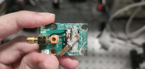 Top view of the EOM, showing (from left to right) the coaxial socket, the capacitor, the copper plate on the top of the Failed to parse (SVG (MathML can be enabled via browser plugin): Invalid response ("Math extension cannot connect to Restbase.") from server "https://wikimedia.org/api/rest_v1/":): {\displaystyle \ce{LiNbO3}} crystal, and the solder pad to which it should be attached (and a lot of damage and excess silver epoxy).
 -
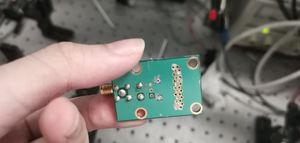 The bottom of the EOM, showing the solder mounds for the coaxial socket, the capacitor, the wire that connects to the top of the EOM, and the base of the solder pad that the crystal is supposed to be on.


The Failed to parse (SVG (MathML can be enabled via browser plugin): Invalid response ("Math extension cannot connect to Restbase.") from server "https://wikimedia.org/api/rest_v1/":): {\displaystyle \ce{LiNbO3}} crystal acts as a capacitor. The top and bottom surfaces of the crystal are coated in gold to ensure a uniform electric field throughout the crystal. Considering the crystal as a parallel plate capacitor, any gaps between the crystal and the "conducting plates" would change the capacitance over those gaps, resulting in an uneven electric field and therefore an uneven phase shift for different parts of the beam, reducing visibility.
However, the crystal had been disconnected from the board by previous users. The connections between the crystal, plate, and board were all made using silver epoxy, which consists of conductive silver dissolved in an organic solvent at room temperature. The advantage of silver epoxy over solder is that we can avoid subjecting the crystal to heat stress from a soldering iron, which may cause it to fracture. It was therefore necessary to reattach the crystal to the board using silver epoxy.
The attempt to repair the EOM board was fraught with misadventures and consumed a significant amount of time. In brief summary:
- The only silver epoxy we found expired 5 years ago and had dried up into solid lumps. We were able to dissolve the dried epoxy using organic solvents and attempt to reapply it to the crystal, but this was a messy affair and the joints formed were not mechanically stable (or at least, not stable enough to survive the various mishaps that occurred after the joints were formed, such as the board being dropped, or other adjustments being made to the board subjecting the joints to too much stress)
- A new replacement epoxy was eventually procured, which, in comic contrast to the solidified old epoxy, was too liquid. Attempts to hasten the binding process using hot air to evaporate the solvent did not succeed, and the liquid epoxy was even more messy. The ultimate solution was to leave the solvent in place with a weight pressing down on it, and to let it slowly evaporate.
- In another ironic twist, after finally fixing the crystal to the board after one month of effort, an adjustment being made to the wire connected to the top plate caused the plate to break off from the crystal. Fortunately, we had learnt our lesson from previous attempts to fix the crystal to the board, and the plate was reattached promptly using the epoxy (although we still had to wait a few days for the solvent to evaporate).
- The messiness of the epoxy was not merely cosmetic: it occluded the optical surfaces of the crystal and formed short circuits between the top and bottom plates. Fortunately, the epoxy does not adhere very strongly to the board or the crystal (adhering instead to metallic surfaces like the gold paint and the solder pads on the board), and was able to be scraped off places where it did not belong.

The repair of the board was not the end of our troubles. It is also difficult to align properly, because the solder mounds on the underside of the board make it difficult to seat the board firmly on the optical mount, while the tension in the coaxial cable used to supply the voltage also makes the system very unstable. Initial attempts to fix the position of the board by pressing it down with a wedge met some success, but it was still too prone to being misaligned while the setup was being adjusted.

Fortunately, the holes in the board are, by coincidence, mostly aligned with the holes in the mount. Although the mount uses imperial-sized screws, we were able to find the screws and components necessary to fix the board in place securely, producing the rather ugly assemblage pictured below.
We also elected to place the board on a mount permitting the pitch and roll of the board to be adjusted, because it is difficult to guarantee its alignment otherwise, and since the crystal is birefringent, we want to ensure it is aligned with the polarisation of the laser, so that the whole beam will experience the same phase difference, and the fringe visibility can be maximised.
We also needed to align the yaw of the EOM. However, given the irregularity of the setup, we could not find a way to do this reliably. We simply tried to ensure the mount was aligned to the grid by visual inspection, and hoped that the error would not be too substantial.
Finally, in order to align the translation of the EOM, we first placed it slightly lower than ideal, allowing the beam to strike the top plate. This created a red spot on the top plate that was used to check the lateral position of the EOM, before the height of the EOM was adjusted. By observing the red spot created on Failed to parse (SVG (MathML can be enabled via browser plugin): Invalid response ("Math extension cannot connect to Restbase.") from server "https://wikimedia.org/api/rest_v1/":): {\displaystyle M_1} , we could see the spot being cut off by the straight edges of the crystal, and adjusted its height so that the spot would sit in between the two straight edges, with minimal occlusion.
Lens and Photodiode Alignment
Lastly, we had to pass the beam through a lens in order to magnify the interference pattern, and finally to align the photodiode to the interference pattern. As shown in the theory section, it is optimal for the screen, which in this case is the photodiode, to be parallel to Failed to parse (SVG (MathML can be enabled via browser plugin): Invalid response ("Math extension cannot connect to Restbase.") from server "https://wikimedia.org/api/rest_v1/":): {\displaystyle M_1} . Since these two components are effectively standalone, it was not difficult to align them to the grid of the table, to which the other components had been aligned, ensuring the formation of circular fringes.
However, the lens was only used to magnify the beam in order to see the features of the interference pattern more closely. For our actual measurements of voltage, we simply directed the beam onto the photodiode to capture as much of it as possible. The pattern after being refracted by the lens was too large to fit entirely on the photodiode.
Results & Discussion
Apparatus Parameters
We are using a Hamamatsu S5106 Si PIN photodiode as our detector, operated at 10V, with a resistive load of Failed to parse (SVG (MathML can be enabled via browser plugin): Invalid response ("Math extension cannot connect to Restbase.") from server "https://wikimedia.org/api/rest_v1/":): {\displaystyle 1~\mathrm{M\Omega}} . Measurements are taken with a Kenwood CS-5270 oscilloscope with Failed to parse (SVG (MathML can be enabled via browser plugin): Invalid response ("Math extension cannot connect to Restbase.") from server "https://wikimedia.org/api/rest_v1/":): {\displaystyle \Delta f = 100~\mathrm{MHz}} and an input impedance of

The Failed to parse (SVG (MathML can be enabled via browser plugin): Invalid response ("Math extension cannot connect to Restbase.") from server "https://wikimedia.org/api/rest_v1/":): {\displaystyle \ce{LiNbO3}} crystal is 3.2mm wide and tall (square cross-section) and 2cm long. The laser pointer lens has a diameter of 3mm, and the wavelength is claimed to be 650nm ± 10nm. We also had access to a pinhole of diameter 1mm.
Michelson Interferometer Fringes
The fine adjustment of the pitch and yaw of the mirrors using the knobs on their optomechanical mounts allowed us to explore the variation in fringe patterns as the mirrors rotate through their angular range of motion. Although our cameras were not able to resolve the details of the interference fringes, we were able to make a few qualitative observations of the fringes formed, using a piece of white paper as a screen:
- It is difficult to tell if the fringes are truly circular, since there may be only one fringe when the mirrors are highly aligned, and it is not possible to tell if the fringe is truly circular or simply the result of viewing very widely separated fringes through a circular aperture.
- Leaving one mirror stationary, say Failed to parse (SVG (MathML can be enabled via browser plugin): Invalid response ("Math extension cannot connect to Restbase.") from server "https://wikimedia.org/api/rest_v1/":): {\displaystyle M_1} , and aligning Failed to parse (SVG (MathML can be enabled via browser plugin): Invalid response ("Math extension cannot connect to Restbase.") from server "https://wikimedia.org/api/rest_v1/":): {\displaystyle M_2} to it would produce a larger number of fringes. Adjusting Failed to parse (SVG (MathML can be enabled via browser plugin): Invalid response ("Math extension cannot connect to Restbase.") from server "https://wikimedia.org/api/rest_v1/":): {\displaystyle M_1} slightly, then adjusting again Failed to parse (SVG (MathML can be enabled via browser plugin): Invalid response ("Math extension cannot connect to Restbase.") from server "https://wikimedia.org/api/rest_v1/":): {\displaystyle M_2} to coincide with it, would be required to produce fringes that were closer to being (what we believe to be) circular, which have only around one fringe and experience large variation in intensity over the variation in Failed to parse (SVG (MathML can be enabled via browser plugin): Invalid response ("Math extension cannot connect to Restbase.") from server "https://wikimedia.org/api/rest_v1/":): {\displaystyle \delta} .
- As the beams became more and more coincident, the fringes seemed to rotate, while increasing in thickness and decreasing in number. After crossing each other, and as they became less coincident, the process was reversed: the fringes continued rotating, but decreased in thickness and increased in number, until they were no longer visible.
Our observations agree with our theoretical derivations. We first consider the case where the mirrors are aligned to each other, although possibly not to the screen, which can be visually verified from the overlap of the beams. In such a case, Failed to parse (SVG (MathML can be enabled via browser plugin): Invalid response ("Math extension cannot connect to Restbase.") from server "https://wikimedia.org/api/rest_v1/":): {\displaystyle \theta_1 = \theta_2} and we have Failed to parse (SVG (MathML can be enabled via browser plugin): Invalid response ("Math extension cannot connect to Restbase.") from server "https://wikimedia.org/api/rest_v1/":): {\displaystyle \begin{align} s &= 2|\delta\cos\theta_1| \\ \psi &= \arctan\left(\frac{1}{\cos\theta_1}\right) = \frac{\pi}{2} - \theta_1 \\ \therefore \Delta d &= 2|\delta\cos\theta_1|\left( \cos\theta_1 \cos\theta + \sin\theta_1 \sin\theta \cos\phi \right) + O(s^2/d^2), \end{align} } which tells us that increasing the misalignment Failed to parse (SVG (MathML can be enabled via browser plugin): Invalid response ("Math extension cannot connect to Restbase.") from server "https://wikimedia.org/api/rest_v1/":): {\displaystyle \theta_1} from the screen makes the fringes straighter and less circular, which means it is not enough to align the beams to each other: they must also be aligned to the screen. However, such a misalignment also reduces the value of , decreasing the spatial frequency and therefore increasing the size of the fringes. This makes it more difficult to judge if the fringes are truly circular when the mirrors are aligned to each other.
However, for the variation in the fringes as the beams cross each other, we were not able to find a convincing theoretical explanation. The rotation of the fringes could perhaps be explained by the maxima and minima shifting with variation in Failed to parse (SVG (MathML can be enabled via browser plugin): Invalid response ("Math extension cannot connect to Restbase.") from server "https://wikimedia.org/api/rest_v1/":): {\displaystyle \psi} , but the expressions for Failed to parse (SVG (MathML can be enabled via browser plugin): Invalid response ("Math extension cannot connect to Restbase.") from server "https://wikimedia.org/api/rest_v1/":): {\displaystyle s} and Failed to parse (SVG (MathML can be enabled via browser plugin): Invalid response ("Math extension cannot connect to Restbase.") from server "https://wikimedia.org/api/rest_v1/":): {\displaystyle \psi} in terms of Failed to parse (SVG (MathML can be enabled via browser plugin): Invalid response ("Math extension cannot connect to Restbase.") from server "https://wikimedia.org/api/rest_v1/":): {\displaystyle \theta_1} and Failed to parse (SVG (MathML can be enabled via browser plugin): Invalid response ("Math extension cannot connect to Restbase.") from server "https://wikimedia.org/api/rest_v1/":): {\displaystyle \Delta \theta = \theta_2 - \theta_1} are too complicated for us to extract meaningful insight from, even with series expansions and other approximations.
Voltage Readings
Even before fixing the EOM, we were able to observe a quantifiable change in the voltage produced with variations in the phase of the interferometer after it was aligned to produce large or circular fringes. The video below shows the variation in intensity of the interference pattern magnified by a lens, while one of the mirrors was being tapped. File:HomodyneDetection IntensityTapping.mp4
There is a 10V difference in measured voltage between points in time where the beam is blocked, and when it is unblocked, as shown in the video below. File:HomodyneDetection FullIncident.mp4
Placing pressure on and tapping one of the mirrors shifts the phase of the beam, changing the intensity of the interference pattern. The variation in intensity only spanned 7V, providing quantitative evidence of an incoherent component in the light contributing the remaining 3V, which we observed visually in the interference. File:HomodyneDetection FullTapping.mp4 File:HomodyneDetection FullPressure.mp4
However, we also observed an unusual variation in the signal at some points. This behaviour would come and go inexplicably, and we are unsure what causes it. We also observed that, upon being switched on, the laser would sometimes vary its phase at a constant rate, creating a shifting interference pattern. This unusual behaviour resolved after restarting the power supply, but we are also unsure what causes it.
File:HomodyneDetection AutoVariation.mp4
We now estimate the noise in our detector system. The effective input impedance, from the resistive load of Failed to parse (SVG (MathML can be enabled via browser plugin): Invalid response ("Math extension cannot connect to Restbase.") from server "https://wikimedia.org/api/rest_v1/":): {\displaystyle 1~\mathrm{M\Omega}} and the input impedance of Failed to parse (SVG (MathML can be enabled via browser plugin): Invalid response ("Math extension cannot connect to Restbase.") from server "https://wikimedia.org/api/rest_v1/":): {\displaystyle 1~\mathrm{M\Omega}} being connected in parallel, is Failed to parse (SVG (MathML can be enabled via browser plugin): Invalid response ("Math extension cannot connect to Restbase.") from server "https://wikimedia.org/api/rest_v1/":): {\displaystyle 0.5~\mathrm{M\Omega}} . First, we consider the shot noise. As previously discussed, the rms current of the shot noise is given by Failed to parse (SVG (MathML can be enabled via browser plugin): Invalid response ("Math extension cannot connect to Restbase.") from server "https://wikimedia.org/api/rest_v1/":): {\displaystyle \left\langle i^2_N \right\rangle=2q_e\bar{i}\Delta f} , where is the average photocurrent that is given by Failed to parse (SVG (MathML can be enabled via browser plugin): Invalid response ("Math extension cannot connect to Restbase.") from server "https://wikimedia.org/api/rest_v1/":): {\displaystyle \bar{i} = \left\langle I \right\rangle A \eta q_e/h\nu} . The maximum voltage (with the zero reference being the voltage reading when no light is incident) is 10V, meaning the detected power is Failed to parse (SVG (MathML can be enabled via browser plugin): Invalid response ("Math extension cannot connect to Restbase.") from server "https://wikimedia.org/api/rest_v1/":): {\displaystyle 2.0 \times 10^{-4}~\mathrm{W}} , since by Ohm's law Failed to parse (SVG (MathML can be enabled via browser plugin): Invalid response ("Math extension cannot connect to Restbase.") from server "https://wikimedia.org/api/rest_v1/":): {\displaystyle P = V^2/R} . This gives us Failed to parse (SVG (MathML can be enabled via browser plugin): Invalid response ("Math extension cannot connect to Restbase.") from server "https://wikimedia.org/api/rest_v1/":): {\displaystyle \bar{i}=1.046 \times 10^{-5}} and therefore, Failed to parse (SVG (MathML can be enabled via browser plugin): Invalid response ("Math extension cannot connect to Restbase.") from server "https://wikimedia.org/api/rest_v1/":): \left\langle i^2_N \right\rangle=3.352 \times 10^{-15} , giving a noise voltage of Failed to parse (SVG (MathML can be enabled via browser plugin): Invalid response ("Math extension cannot connect to Restbase.") from server "https://wikimedia.org/api/rest_v1/":): {\displaystyle 4.09 \times 10^{-2}~\mathrm{V}} .

We next consider Johnson noise. Through the equation Failed to parse (SVG (MathML can be enabled via browser plugin): Invalid response ("Math extension cannot connect to Restbase.") from server "https://wikimedia.org/api/rest_v1/":): {\displaystyle \left\langle i^2_N \right\rangle=4k_BT\Delta f/R} , we find a current of Failed to parse (SVG (MathML can be enabled via browser plugin): Invalid response ("Math extension cannot connect to Restbase.") from server "https://wikimedia.org/api/rest_v1/":): \left\langle i^2_N \right\rangle=1.646 \times 10^{-18} at a room temperature of . This gives an rms voltage of Failed to parse (SVG (MathML can be enabled via browser plugin): Invalid response ("Math extension cannot connect to Restbase.") from server "https://wikimedia.org/api/rest_v1/":): {\displaystyle 9.07 \times 10^{-4}~\mathrm{V}} .

Lastly, while the definition of the GR noise requires detailed knowledge of the electron-hole recombination process, it has estimated by the manufacturer as the noise-equivalent power or NEP in the datasheet. This is given as Failed to parse (SVG (MathML can be enabled via browser plugin): Invalid response ("Math extension cannot connect to Restbase.") from server "https://wikimedia.org/api/rest_v1/":): {\displaystyle 1.6 \times 10^{-14}~\mathrm{W}~(\mathrm{Hz})^{-1/2}} , giving us an rms noise voltage of Failed to parse (SVG (MathML can be enabled via browser plugin): Invalid response ("Math extension cannot connect to Restbase.") from server "https://wikimedia.org/api/rest_v1/":): {\displaystyle 1.3 \times 10^{-2}~\mathrm{V}} .
Remarkably, despite the simplicity of our setup, the dominant source of noise in this setup is shot noise—we have managed to build a shot-noise limited detector. All sources of noise (aside from the inexplicable low-frequency noise) are several orders of magnitude lower than the variation in voltage from phase changes, implying that this system can be used effectively for modulating and transmitting information.
Laser Beam
Despite the process of measuring the laser spot size being rather straightforward to describe, we did not have the equipment to perform a sufficiently precise characterisation. An attempt was made by sliding a box along the edge of a folded piece of paper, with the intention to mark the position of the box on the piece of paper and record the corresponding intensity. However, the lack of rigidity of the apparatus, the lack of precision of our measurement instruments (a pen and a ruler), a lack of manual dexterity and a lack of time to work around these problems made this infeasible.

Further, as is visible from our images, our beam profile is nowhere close to Gaussian, and instead rather jagged and irregular. One possibility for cleaning up the signal was to send it through a small circular pinhole first. Indeed, by doing so, we were able to observe an Airy disk. However, due to the aperture being much smaller than the beam, a significant fraction of the light was lost. The resulting photocurrent only induced a maximum of a little over 2V, as compared to 10V with the full beam being used. The interference patterns formed were also less visible, so we did not primarily rely on this method to perform our observations.
File:HomodyneDetection PinholeIncident.mp4
However, we were able to induce a larger variation in the voltage, consisting of almost the full 2V, by placing pressure on the mirror and thereby inducing phase variations.
File:HomodyneDetection PinholePressure.mp4
Phase Modulation
Having thus established our interferometer, we now proceed to the second major aspect, which is to control the phase, and therefore the received photocurrent and measured voltage. A major issue we faced is that the Failed to parse (SVG (MathML can be enabled via browser plugin): Invalid response ("Math extension cannot connect to Restbase.") from server "https://wikimedia.org/api/rest_v1/":): {\displaystyle \ce{LiNbO3}} crystal we obtained, and the EOM board it came with, was not characterised. In fact, while the crystal was cuboidal in shape, we were unsure if the long axis along which light would generally be transmitted was the optic axis or not. A further complication is that we do not have an extra crystal to compensate for birefringence, so if the long axis is not the optic axis, we would instead have to resort to trying to ensure the crystal and laser are aligned, to ensure the coherence is minimally disrupted by birefringence.

Despite our best efforts, we were not able to perfectly align the EOM board. The Failed to parse (SVG (MathML can be enabled via browser plugin): Invalid response ("Math extension cannot connect to Restbase.") from server "https://wikimedia.org/api/rest_v1/":): {\displaystyle \ce{LiNbO3}} crystal's optical surfaces seem to be somewhat reflective, producing an additional red spot on the screen. The spot was confirmed to be produced by the crystal by blocking the two mirrors and observing that the spot is still there, whereas it disappears if light from Failed to parse (SVG (MathML can be enabled via browser plugin): Invalid response ("Math extension cannot connect to Restbase.") from server "https://wikimedia.org/api/rest_v1/":): {\displaystyle B_1} is not allowed to reach the crystal. If the setup was perfectly aligned, this additional spot would have formed exactly at the position of the beam that reflected from Failed to parse (SVG (MathML can be enabled via browser plugin): Invalid response ("Math extension cannot connect to Restbase.") from server "https://wikimedia.org/api/rest_v1/":): {\displaystyle M_1} , but this was not the case. While this additional spot is not visible in the image, a similar effect produces the additional misaligned spot on Failed to parse (SVG (MathML can be enabled via browser plugin): Invalid response ("Math extension cannot connect to Restbase.") from server "https://wikimedia.org/api/rest_v1/":): {\displaystyle M_1} , this time caused by the beam, reflected by Failed to parse (SVG (MathML can be enabled via browser plugin): Invalid response ("Math extension cannot connect to Restbase.") from server "https://wikimedia.org/api/rest_v1/":): {\displaystyle M_1} , hitting the crystal. While some light is transmitted onwards to the screen, some is reflected, forming the additional spot on .
While the additional spot sometimes displays visible fringes, it does not interfere with the beam from Failed to parse (SVG (MathML can be enabled via browser plugin): Invalid response ("Math extension cannot connect to Restbase.") from server "https://wikimedia.org/api/rest_v1/":): {\displaystyle M_2} when said beam is overlapped onto it. That the fringes arise from interference can be verified by applying a slight pressure to the EOM board, which produces a shift in the pattern characteristic of interference. One possibility is that the path difference between this path reflecting from the EOM, and the path reflecting from Failed to parse (SVG (MathML can be enabled via browser plugin): Invalid response ("Math extension cannot connect to Restbase.") from server "https://wikimedia.org/api/rest_v1/":): {\displaystyle M_2} , exceeds the coherence length of the low-qualtiy laser. However, the laser claims to have a wavelength of 650nm ± 10nm. If that was truly the case, then the coherence length would be would be Failed to parse (SVG (MathML can be enabled via browser plugin): Invalid response ("Math extension cannot connect to Restbase.") from server "https://wikimedia.org/api/rest_v1/":): {\displaystyle \ell_c \approx \frac{c}{\Delta \nu} = \frac{1}{\lambda_{\min}} - \frac{1}{\lambda_{\max}} = 4.7 \times 10^4~\mathrm{m}, } far greater than the size of our experiment. It may be possible that the bandwidth stated on the laser is not truly the bandwidth, but the uncertainty in the average frequency, or it may be that the light is somehow being scattered incoherently before landing on the screen. Additionally, it is unclear what this reflected beam is interfering with.
A far worse problem, however, was discovered very close to the end of the project. Despite all the effort put into repairing the EOM board, the coaxial socket does not seem properly connected to the top plate, and even worse, there seems to be a short circuit within the coaxial socket. This was first suspected when it was observed that driving the EOM with a function generator through a high voltage amplifier did not produce any change whatsoever in the observed voltage when the signal was switched on and off, and strongly suspected when it was observed that a high voltage power supply would have its output drop to 0V when connected to the EOM. These faults were confirmed by direct measurement of resistance using a multimeter, which discovered these faults.
- Resistance Measurements
-
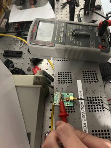 An open circuit with infinite resistance between the inner receptacle of the coaxial cable and the top plate of the crystal.
 -
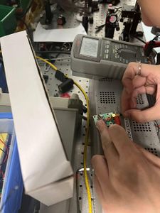 A short circuit with finite resistance between the inner receptacle of the coaxial cable and its housing. The value of the resistance fluctuates significantly.


In the course of trying to repair the EOM board, we had attempted to desolder the coaxial socket and transfer it to a new board, or else use a new coaxial socket with a new board. Comically, but very unfortunately for our experiment, despite there being a vast number of similar boards and coaxial sockets in the drawers at the CQT Workshop, none of the coaxial sockets can fit in any of the new boards, and the socket that we have, which definitely fits, seems resistant to desoldering (the solder on its legs did not melt even after being exposed to a soldering iron at 450 °C). Having exhausted these options (and the crystal breaking off from the board again shortly after this discovery, for good measure), it was decided to admit defeat and limit ourselves to presenting these results and observations, instead of trying again to get our phase modulation to work.
Conclusion
In the course of this project, we analysed and built a Michelson interferometer from an assortment of optomechanical components and a laser pointer. We have learnt various practical skills relating to the improvised construction of mounts and electrical systems, the assembly of components using specialised materials, and the alignment of optical components. We have also performed a theoretical analysis and qualitatively confirmed some of our predictions, and surprisingly managed to construct a shot-noise limited detector.
Nonetheless, despite extensive effort, we were unable to repair the EOM, due to an electrical fault in the socket. While we had thought to check the electrical connectivity of the rest of the circuit, we did not expect that there would be issues with the socket. This is a learning point to check all parts of each component carefully, especially if they are of dubious provenance.
In conclusion, I'm really glad I'm a theorist.