Characterization of Single Photon Counters

Characterization of APDs. Proposed by zhen yuan.

Brief background

Count single photons using the photoelectric effect. In simple terms, there is a semiconductor part and an electronics & signal processing part. The semiconductor part is responsible for converting the incident photon into a photoelectron-hole pair and accelerating them to create a cascading effect which amplifies the photocurrent. The peripheral electronics are responsible for measuring these peaks as well as restoring the bias voltage for subsequent detection events. The electronics are also needed to turn that analogue signal into digital signals for a computer to process further.

Key Objectives

- Automate the recording of oscilloscope frames. (To allow for further processing via a computer)

- Quantify the timing jitter of those frames. (Temporal consistency of oscilloscope frames)

- Characterization of APD (Overvoltage, dark count rate and mean peak heights. SAP500 used)

- Response of APD to photons from LED (Differences between "dark" peaks and peaks from LED photons)

Timing Jitter Of Digital Oscilloscope (model: GDS1072B)

The automated recording of Oscilloscope frames is presumably limited by the baud rate. The reason is that the Oscilloscope is capable of sampling at 1 billion samples per second, assuming samples are 8 bits (discrete values between -128 & 127 inclusive), resulting in 1 gigabyte per second of data transfer. The baud rate used was 1152000B or about 1 megabyte per second.

A natural question is: what is the timing jitter of the "frames" that are recorded on the computer? Are the frames arriving at a constant rate? What is the deviation of the arrival times?

To quantify this uncertainty, a known signal was generated (using a function generator) and the frames are recorded as usual. The time of arrival of frames could be inferred by fitting the values of the frames to the known signal.

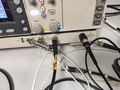
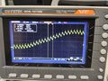
[FIG] (Left): Experimental setup. (Right): Oscilloscope during the data collection.

[FIG] (a): Sequentially arrived frames represent a sample of the generated waveform. For this plot, a 1Hz sine function was used. (b): The initial fitting of the sine function allows the determination of the frequency of the arrival of frames. The data points are fitted with python's `scipy.optimize.minimize` routine where the horizontal scaling and offset was fitted for.

[FIG] (a): Here a Zigzag waveform was used since the slope is supposed to be constant between the peaks and troughs of the waveform. The frames that are near the peaks and troughs are not used for the line fitting because it may be difficult to identify which line frame corresponds. (b): The fitted line as well as the corresponding coefficient of determination is shown. (c): The average value of the frame obtained is plotted onto the fitted lines. See the next figure for a close-up view.

[FIG] (a): Close up view of the fitted line and the averaged frame value. Inset shows the calculation of the timing jitter of a particular frame. (b): Histogram of the timing jitters of each frame over 71 frames of data. The average absolute jitter is about 500ns while the maximum jitter is about 1400ns.

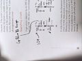
[FIG] Schematic of serial communication via USB connection to the oscilloscope. The left schematic shows the existing communication protocol between the computer and the oscilloscope. The right schematic shows an asynchronous version which could improve the number of frames collected per unit time. However, this schematic was not implemented for this experiment.

[DISCUSSION] There are several factors that may affect the timing jitter of the oscilloscope. The read/write speed of the computer as well as the availability of the I/O process of the computer may be the 2 most important factors. This is because the next frame of data is requested after the computer is done saving the previous frame (see serial communication schematic). The write speed is dependent on the computer disk, which may be between 1MB/s (HDD) to 100MB/s (SSD), and also other computer processes which may be using the disk at the time of data capture. One possibility is to save the data asynchronously as shown in the right schematic, however, this option is not explored for this study.

Experimental Discussion/Results: Overvoltage Characterization (result06)

A simple characterization of the APD was done. APD used was SAP500 with a passive quenching setup with shielding from external light sources. The breakdown voltage, $V_{br}$, was determined by slowly increasing the applied reverse bias voltage, $V_{rb}$, and stopping when peaks are first observed from the APD. The breakdown voltage was determined to be 139.3$\pm$0.1V. Overvoltage, $V_{ov}$, is defined as $V_{ov}=V_{rb}-V_{br}$. The current from the APD was collected as a function of overvoltage and we expect the peaks of the APD current to be higher when the overvoltage is higher.

[FIG] Typical signal from APD at different overvoltages. Peaks were detected using python's `scipy.signal.find_peaks`.

[FIG:ref06_02] Peak heights of APD signal VS overvoltage. This trend is the same as expectations. Interestingly, the standard deviation (error bars) also increases with increasing overvoltage. The scatter plot shows the individual peak heights. Note: $n$ refers to the number of peaks detected (dark counts) within 100 frames. Each frame lasts for 0.5 milliseconds. See below for dark count rate.

[FIG] Dark count rate VS overvoltage. This trend is the same as expectations. The dark count rate (cps) is of the same magnitude as the SAP500's datasheet.

[DISCUSSION]: These data were collected using the oscilloscope recording technique proposed earlier. While these statistical data (like mean counts, mean heights, st. dev.) could be obtained from the standalone oscilloscope, obtaining the data points for the scatter plot in FIG:ref06_02 would be impractical (transferring 500 files from the oscilloscope to the computer).

Experimental Discussion/Results: APD counts vs square wave LED voltage (result03)

With the ability to collect lots of frames of the oscilloscope, we are now able to capture frames which are 200 microseconds long with about 8 APD peaks on average. This is interesting because we can use a function generator to power a LED with a square waveform of 64kHz at 20% duty cycle, and observe how the APD responds to these LED photons. The voltage offset of the waveform is increased over time so that at certain offsets, the peak of the square waveform has sufficient voltage for the LED to create photons. The 20% duty cycle is used so that during the 80% downtime, the APD has sufficient time to reset to its ready state.

[FIG] (a): Voltage supplied to the LED from the function generator. (b): Signal obtained from APD. (c-f): Zoomed in portion of APD signal. (f): saturated APD shows multiple after-pulses that are lower than the average single-photon pulse.

[FIG] (Left): Raw Signal from APD. The voltage signal was measured across a 220 Ohm resistor. The APD peaks were determined with python's `scipy.signal.find_peaks`. (Middle): Raw Signal from the LED. The voltage signal was measured directly across an LED. (Right): Determination of the frequency and duty cycle of the LED signal. The "on" and "off" states of the LED were determined with thresholding. The frequency was determined by finding the average period between "on" states and using the formula frequency=1/period. The duty cycle was determined by the ratio of the average number of "on" states to the average number of "on" and "off" states.

[FIG] The LED voltage was step-wise increased at every 500th frame. At about the 9000th frame, the APD was believed to be saturated and hence the voltage was step-wise decreased instead. The decrease in LED voltage allows for some hysteresis check. (a): Number of APD peaks per frame VS frame id. (d): Peak LED voltage. Note that only the peak of the square waveform is shown. (b,c,e,f): Zoomed in versions of (a) and (d). (e): Shows the step-wise increase at 500th frame. However, in practice, this voltage change is done manually, hence there is a slight delay before the voltage is finally stable at the new height.

[FIG] (a): Peak LED voltage with intermediate transient voltages. (b): Peak LED voltage when it is stable. Frames with transient voltages were removed by skipping the 1st-100th frame at every 500 frame intervals. This leads to 400 useful frames per 500 frame intervals. (c): Number of APD peaks or counts in each frame. Only selected data was shown to prevent clutter. Here we see that increasing the LED voltage increases the number of APD peaks. (d): Scatter plot of APD counts VS LED voltage. Increasing LED voltage generally increases APD counts. However, when APD is saturated, the APD counts decrease. The orange points are for lowering LED voltage and they correspond well to the points for increasing LED voltage. While this suggests that there is no hysteresis against increasing or decreasing LED voltage, more data points would be needed since there are only 2 data points where the LED voltage is decreasing.

[FIG] Dark noise analysis of APD. (a): A typical frame when LED voltage is not enough to generate photons. Coloured lines show the relative difference in height and durations between consecutive APD peaks. (b): Scatter plot of differences in APD peaks and intervals. (c): Histogram of the differences in consecutive peak heights. This distribution is relatively symmetric. (d): Histogram of the number of counts per frame. This histogram is expected to be Poissonian assuming that the arrivals of the photons are memory-less.

Types of poissonian distributions.

For comparison, a simulated Poisson distribution with the same average count was drawn. The dark counts from the APD have a variance that is smaller than an ideal Poissonian distribution with the same mean. This sub-Poissonian distribution is unexpected if the APD peaks are truly memoryless. It is likely that some of the peaks observed are correlated, for example, after pulses. (e): The histogram of the duration between consecutive peaks. This was supposed to follow an exponential decay curve $e^{-\lambda \Delta t}$. However, due to the dead time of the APD, it is very unlikely for a peak to be detected during this period. (f): An exponential function was fitted to the histogram in (e) using python's `scipy.optimize.curve_fit`. Points after the maximum are used for this fitting. The dead time of the APD was estimated to be 10 microseconds. This is likely to be a large overestimation (upper limit) of the APD's dead time.

[DISCUSSION] The dead time could be theoretically calculated using the formula: $\tau =RC$. For this experiments, the values used are $R=560$kOhm and $C=3.3$pF, the calculated time constant, $\tau =1.85\approx 2$ microseconds. This value is closer to the expected dead time typical for this APD (SAP500) under passive quenching mode. However, experimentally, there are rarely any APD peaks within 10 microseconds of an initial peak. This indicates that the theoretically calculated dead time is too idealistic most of the time.

Updates/Progress/Changelog

• 8 Feb 2022:

* Fabrication may not be possible with current resources.
* Instead, we will focus on characterizing existing APDs or photodiodes that are available.
* Seems that there exist some possibly faulty or broken setups of APDs, we may look to troubleshoot them.
* Example of APD characterization done by FYP student from CQT & masters thesis on the same topic .
* From the PDF, it seems that the avalanche "pulse" can be measured directly. This begs the question: how does the shape of the pulse correlate to the photon counts?
* Problem posed by Christain: How are single photons defined/characterized?

• 11 Feb 2022:

* got a working signal from the "homemade" APD! 
* Next is to lower the light intensity of the LED and measure the signal from the APD as a function of LED power.

• 15 Feb 2022:

* attempted to connect GDS 1072B to laptop. tried the driver, but the oscilloscope could not be detected. 
* will look into the source to debug the driver.
* able to retrieve the data via thumb drive.
* Signal from homemade APD is a negative logic signal. It turns on when a photon causes an electron avalanche. (this is not what we need for the characterization)
* Next, will be using the APD testing kit to test the raw APD.

• 18 Feb 2022:

* Could not get the APD kit to work. Suspect its because of an open circuit on the board (unsure if this was intended or not).
* the high voltage DC-DC converter seems to be functioning properly and responsive to control voltage.

• 4 Mar 2022:

* traced and compared schematic to the actual board. slight discrepancies found.
* However, now the plan is to use the DC-DC converter directly to supply high voltage to the APD and measure the response to light.
* The APD is shown to respond to light as expected. 
* Next step is to figure out a way to supply a controlled amount of light and correlate this with the response from APD.
* Also, there is a need to understand the response from APD.

• 11 Mar 2022:

* recreated APD schematic from data sheet.
* The bare APD is shown to respond to light as expected. 
* May have burnt out APD from the previous step due to lack of resistor.

• 15 Mar 2022:

* Finally able to retrieve data directly from GDS 1072B ( GDS1072B )
* Installation of the driver is described for others.
* found an opensource python interface for the oscilloscope.
* Next step is to allow for continuous data collection.

Current goals

Obtain enough setup to measure a pulse from an APD. For example:

Setup

• "test" setup:
  • photon source >> laser attenuator >> APD >> ADC >> Raspberry Pi

• control setup:
  • photon source >> laser attenuator >> "Professional" SPCM >> ADC >> Raspberry Pi

Equipment needed

Semiconductor device:

• May need a semiconductor fabrication facility with the ability to make thin films on Silicon.
• A photodiode or APD to see how it performs.

Analog electronics:

• Circuit design to convert analog signal to digital signal.

Prebuild devices/hardware:

• laser source or photon source
• laser attenuator
• computer/Raspberry Pi for data processing
• Analog to Digital Converter (ADCs)
• "Professional" grade Single Photon Counting Module (SPCM) to characterize experimental setup.
• Fast oscilloscope.

tl;dr wishlist:

• Avalanche Photodiodes (need any 1)

  

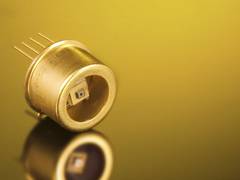
  A picture of an APD. SAP series

  • Laser Components SAP500 (passive)
  • Perkin Elmer C30902SH (passive)
  • Perkin Elmer SPCM-AQR-15 (active)
  • MPD PD-050-CTD-FC (active)

• APD testing kit
• Laser source
• Photon attenuator
• Computer/Raspberry Pi for data processing

Potential Problems

• Dark noise may be overwhelming, so we may need to find a way to suppress it. (I suspect this is why commercial devices cost $2k-5k)
• Fabrication cost of the custom semiconductor device may be too high or impractical... gg.com (or we just refurbish an LED/solar panel, this will have lower PDE, but maybe we can use electronics to maximise the PDE.)
• Electronic circuitry costs. (Unlikely to be too costly)

Gallery

11 Feb:

• 
  NIM pulse.
• 
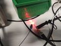  Optic Fiber with led.
• 
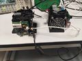
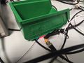  Covered set up.
• 
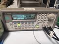  Signal generator to pulse the LED.
• 
  50 Ohms Impedence matching
• 
  APD used
• 
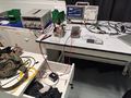
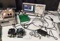  Overview of setup

15 Feb:

• 
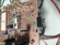
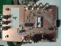  apd testing kit
• 
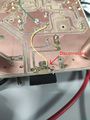
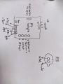  apd testing kit pin outs
• 
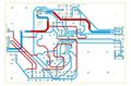
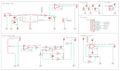  apd testing kit electronics wiring diagram
• 
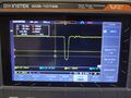
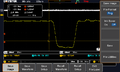  Oscilloscope image of NIM pulse retrieved from thumb drive

18 Feb 2022:

• 
• 
• 
  Could not get the APD kit to work. Suspect its because of an open circuit on the board (unsure if this was intended or not).

4 Mar 2022:

• 
• 
  The APD is shown to respond to light as expected. However, there is still a lack of understanding of the signal received.

11 Mar 2022:

• 
  recreated APD schematic from datasheet.
• 

15 Mar 2022:
GDS 1072 B actual driver must be downloaded from https://www.gwinstek.com/en-global/products/detail/GDS-1000B
You will need an account to download it. navigate to the "hardware and devices panel" to install the driver.
This screenshot is for windows 10, win10. Openwave softwave can be downloaded from github: https://github.com/zhenyuan992/OpenWave-1KB .
Simply git clone and double click on the OpenWave-1KB.exe file

• 
  installation of GDS 1072B driver.
• 
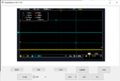  image output from openwave software
• 
  raw data output from openwave softwave