Quantum Random Number Generator

Team Members

Wang Yang A0228753X

Xiao Yucan A0236278W

Zhang Munan A0236273E

Idea

We live in an increasingly connected world, where a superior source of entropy is the key to data security. The effectiveness of any cryptographic system is determined by the strength of the keys it used. In turn, the strength of the key is determined by the degree of randomness used in its generation. Besides, large amount of random numbers are at the core of Monte Carlo simulations, which are widely used in scientific research. Methods produce random numbers from any algorithm are called pseudo-random number generator(PRNG). And random numbers generated by PRNG are deterministic by definition and therefore unsuitable for cryptographic purposes.

In order to generate unpredictable random numbers, hardware random number generators have been widely used. These physically generated random numbers are considered "truly" random because it is either practically or fundamentally impossible to predict the outcome of such a device. Quantum Random Number Generators (QRNGs) belong to a class of hardware random number generators and leverage the random properties of quantum physics to generate a true source of entropy, improving the quality of seed content for key generation.

Early QRNGs were based on radioactive decay. And more recently, QRNGs based on Poisson statistics of photons have been developed. The core idea is shown in the figure below. Single photons generated by a laser source are incident on a semi-transparent mirror and the mutually exclusive events (reflection/transmission) are detected and associated with ‘0’ or ‘1’ bit values respectively. The unpredictability of generated numbers is ensured by the quantum nature of the process. However, such a scheme needs a reliable single photon source as well as single photon detectors and it's not possible for our project. Here, we decided to build a QRNG based on measuring vacuum fluctuations of a light field as a random source. More details will be discussed in the principle part.

Figure 1. Schematic of branching path quantum random number generators

Benefits of having a quantum random number generator

• The source of randomness is unpredictable and controlled by quantum process.
• Live/real-time monitoring of entropy source is possible and highly effective as well.
• All attacks on the entropy source are detectable.

Application of quantum random number generator

• Securing data at rest in data centres
• Securing any kind of sensitive data
• Securing data in the cloud
• One-time pad for authentication in banking and other transactions
• Gaming applications and lottery
• Block-chain network
• Numerical simulations, statistical research
• IoT devices
• E-commerce and banking applications
• Cryptographic applications
• Telecom and 5G
• Monte Carlo Simulation

Principles

Figure 2. Schematic of quantum random number generator based on measuring vacuum fluctuations

Figure 2 schematically shows our setup. Such a setup is known as balanced homodyne detection and can extract the information of the electrical field in the second mode entering the polarizing beam-splitter (PBS) by measuring the photocurrent difference $i_{1}-i_{2}$. A continuous wave laser (wavelength 658 nm) is incident on one input port of the PBS and used as the local oscillator (LO), while another input port is empty. So the homodyne detection is trying to measure the vacuum state of the electromagnetic field. The randomness source in our setup is the fluctuations of the vacuum field. Here we tried to balance the optical power impinging on the two photodiodes, therefore any power fluctuation coming from the laser diode will be detected simultaneously and canceled in the photocurrent difference.

Alternatively, the randomness can be seen as coming from the shot noise of the photocurrents $i_{1}$ and $i_{2}$ with a power proportional to the average optical power. Since the shot noise currents from the diodes are uncorrelated, the noise adds up. And the amplitude fluctuations in the laser intensity (referred to as classical noise) can be eliminated by measuring the photocurrent difference.

Setup

Figure 3. Schematic of setup

The original setup was built with as few components as possible to create a baseline performance that we can compare. A schematic of setup is shown in Figure 3.

Figure 4. Experimental setup

Tool list

① Laser Diode

Laser Diode is powered by a laser driving unit. The light intensity can be changed by changing the laser current.

② Focal Lens

By adjusting the focal length, the intensity of light that finally hits the photodiodes is adjusted.

③ RP: Rotatable Polarizer

The polarization state of the light is adjusted by rotating the polarizer.

④ Mirror 1

By adjusting mirror 1, the position of transmitted and reflected light spots hitting on PD1 and PD2 can be adjusted simultaneously.

⑤ PBS: Polarizing Beam Splitter

The laser beam incident on the PBS can pass through or be reflected depending on the polarization state. If the incident beam is diagonal polarized (45°), the intensity of reflected and transmitted light is equal.

⑥ Mirror 2

By adjusting mirror 2, the position of transmitted light spots hitting on PD2 can be tuned.

⑦&⑧: Photodiodes

Detect the intensity of incident light.

Description

The total light power is changed by changing the laser current and adjusting the focal lens, while the power of the two output ports of the PBS is balanced by rotating the polarizer in front of the laser diode. Light leaving the PBS is detected by a pair of reverse biased photodiodes connected in series to perform the current subtraction. By adjusting the orientation of M1 and M2, the light intensity incident on PD1 and PD2 can be adjusted and balanced. The balancing of the photocurrents is monitored by observing the voltage drop across a resister $R_{DC}$ (DC port). Here we use a multimeter to measure the voltage. The fluctuations $\Delta (i_{1}-i_{2})$

Characterization list

① Oscilloscope

② Spectrum Analyzer

Process

• 26 February 2022:

* Did a basic characterization of photodiode
* Inputted a sine wave signal and a laser pointer light, observed the waveform of the photodiode

• 
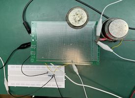  Figure 5. Basic characterization of photodiode test
• 
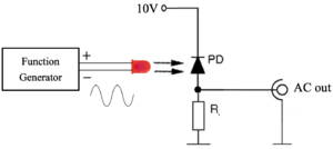  Figure 6. Schematic of basic characterization of photodiode test

To understand the optical response of the photodiode, we used a laser pointer to test its output waveform, because the laser is not periodic, so the waveform is not regular, but there are signals from the oscilloscope.

Then we inputted a periodic sine signal to excite the laser diode to output laser incidents on the photodiode, and it showed a periodic sine signal with a very regular sine waveform. When the frequency increased over 1 GHz, we could not observe a regular and stable waveform.

• 5 March 2022:

* Used different resistors to test the frequency response of photodiode

• 
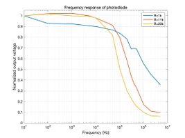  Figure 7. Graph of the frequency response of photodiode

We changed the resistors in Figure 6, from 1 kΩ to 11 kΩ and then 20 kΩ. We found that the higher the resistance of the resistor, the larger the output voltage but less sensitive to the high frequency.

• 12 March 2022:

* Build up the laser system and ensured the laser output

• 
  Figure 8. HL6501MG laser diode and schematic of internal circuit
• 
  Figure 9. Schematic of electronics laser connector circuit
• 
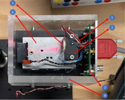  Figure 10. Laser source setup

We used a HL6501MG laser diode, which is a 0.65 μm band AlGaInP laser diode (LD) with a multi-quantum well (MQW) structure. It is suitable as a light source for large-capacity optical disc memories and various other types of optical equipment. Hermetic sealing of the small package (φ=5.6 mm) assures high reliability.

The Laser source consists of ① Laser diode; ② Thermostat; ③ Supply circuit for Laser diode and Thermostat; ④ Shell; ⑤ Focal lens; ⑥ Radiator. The Laser Diode is in the thermostat which is connected to the Radiator. We can set the temperature on the Laser power supply. The Thermostat and Radiator will keep the temperature of the laser diode as same as that set on the laser power supply. There is a focal lens in front of the laser diode. We can use it to change the focal length the enlarge the laser intensity hitting on the photodiodes. And a shell made of acrylic sheet and 4 balance posts.

• 19 March 2022:

* Soldered photodiode driving circuit
* Test the feasibility

• 
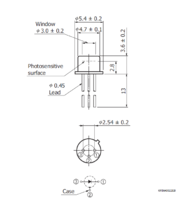  Figure 11. S5972 Si PIN photodiode and schematic of internal circuit
• 
  Figure 12. Principle of photodiode driving circuit
• 
  'Figure 13. Schematic photodiode driving circuit block

We applied an S5972 high-speed Si PIN photodiode for detecting the light, it is designed for visible to near-infrared light detection. These photodiodes provide wideband characteristics at a low bias, making them suitable for optical communications and other high-speed photometry.

We combined two photodiodes in the circuit and soldered them in the circuit chip as Figure 12 shows. After that, we tested its performance by the laser source, it was approved that the optical signal was converted into the electrical signal and was observed by oscilloscope.

• 26 March 2022:

* Build up the whole system
* Tune the bias of two photodiodes

• 
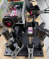  Figure 14. The whole system setup

We built up the whole setup on the optical platform. Then we tuned the bias of two photodiodes to make sure that the intensity of the laser hitting on both photodiodes is the same by adjusting the multimeter's voltage to around 0.

• 2 April 2022:

* Focus the laser output
* Maximize the laser power output
* Characterize varaiation by varying optical power

• 
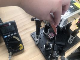  Figure 15. Maximize the laser power output
• 
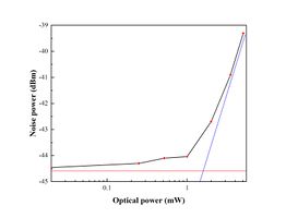  Figure 16. The plot of the detector noise power by varying the incident optical power

We found that the Laser power output in front of the RP is 20 mW. But the power detected by the photodiodes was only 0.4 mW. So, we needed to change the focal length of the focal lens to maximize the laser power output. We blocked one photodiode and the used the output voltage to calculate the output laser power. After lots of tests, we get the maximum value of output voltage, 9.17 V, which means 8.85 mW. Almost half of that detected before the RP.

Then, we characterized the change of noise level while rising incident optical power. And then we plotted a graph which is shown in Figure 16, it is easy to find when the optical power is at a relatively low range, the noise level is flat which corresponds to the horizontal red line. While the optical power rises, the noise level increases proportionally to the optical power. Therefore, we have enough reasons to believe that the overall noise is dominated by electronic noise in the low optical power range, while the noise level is dominated by shot noise and proportional to the optical power in the high optical power range.

• 9 April 2022:

* Soldered high pass filter
* Test its feasibility

• 
  Figure 16. Schematic of high pass filter circuit
• 
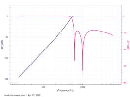  Figure 17. Graph of theoretical high pass filter frequency response
• 
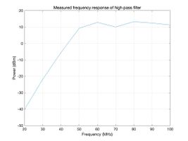  Figure 18. Graph of measured high pass filter frequency response
• 
  Figure 19. Setup of high pass filter
• 
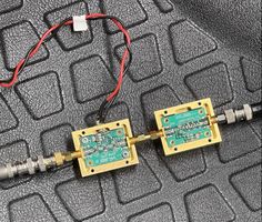  Figure 20. Setup of gain block and high pass filter

The measured total noise has a lot of low-frequency noise and is relatively flat power density in the range of 60-200 MHz. With a low pass filter of 200 MHz in the oscilloscope, we just needed a high pass filter of 60 MHz which compresses the low-frequency fluctuations. So we designed a high pass filter of 60 MHz and soldered the high pass filter.

After that, we tested its performance. By comparing with the theoretical high pass filter graph, the measured high pass filter frequency response showed a high correspondence with it, which means it is feasible to apply it to the whole system to suppress the low-frequency fluctuations.

• 16 April 2022:

* Apply the high pass filter to the circuit and test
* Record data and draw some graphs analysis

• 
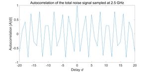  Figure 21. Autocorrelation of the total noise signal sampled at 2.5 GHz
• 
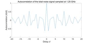  Figure 22. Autocorrelation of the total noise signal sampled at 1.25 GHz
• 
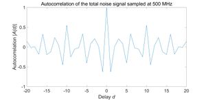  Figure 23. Autocorrelation of the total noise signal sampled at 500 MHz
• 
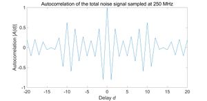  Figure 24. Autocorrelation of the total noise signal sampled at 250 MHz
• 
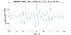  Figure 25. Autocorrelation of the total noise signal sampled at 100 MHz
• 
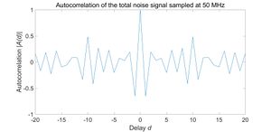  Figure 26. Autocorrelation of the total noise signal sampled at 50 MHz
• 
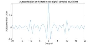  Figure 27. Autocorrelation of the total noise signal sampled at 25 MHz
• 
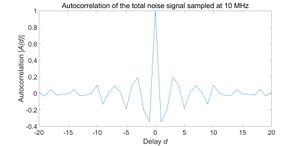  Figure 28. Autocorrelation of the total noise signal sampled at 10 MHz
• 
  Figure 29. Autocorrelation of the total noise signal sampled at 5 MHz
• 
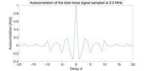  Figure 30. Autocorrelation of the total noise signal sampled at 2.5 MHz
• 
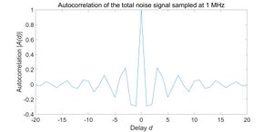  Figure 31. Autocorrelation of the total noise signal sampled at 1 MHz
• 
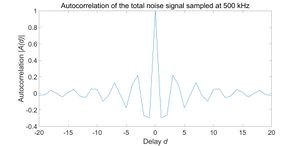  Figure 32. Autocorrelation of the total noise signal sampled at 500 KHz

Codes:(Example of autocorrelation graph at 2.5 GHz)

z7 = highpass(TrigTime10,750000000,2500000000);
[ACF,lags] = xcorr(z7);
plot(lags,ACF./max(ACF),'LineWidth',1);
xlim([-20,20]);
xlabel('Delay \itd','FontSize',25);
ylabel('Autocorrelation |\itA(d)|','FontSize',25);
title('Autocorrelation of the total noise signal sampled at 2.5 GHz','FontSize',25);
set(gca,'FontSize',25);

• 23 April 2022:

* Processing experimental data
* Draw autocorrelation images
* Summarize and upload the experimental results

Results

Quantum noise

• To ensure that the fluctuations at the amplifier output are dominated by quantum noise, the spectral power density is measured (see Fig. on the right).

Fig.？.Amplified noise levels measured into a resolution bandwidth B = 3 MHz

Amplified noise levels measured into a resolution bandwidth B = 3 MHz. The total noise is measured from the photocurrent difference $i_{1}-i_{2}$ with equal optical power impinging on both photodiodes. The current $i_{1}$ of a single photodiode reveals colored classical noise. The electronic noise is measured without any optical input.

In an alternative view, the laser beam can be seen as generating photocurrents $i_{1}$ and $i_{2}$ with a shot noise power proportional to the average optical power. The shot noise currents from the diodes add up as they are uncorrelated, while amplitude fluctuations in the laser intensity (referred to as classical noise) do not affect the photocurrent difference.

Autocorrelation

• Autocorrelation, sometimes known as serial correlation in the discrete-time case, is the correlation of a signal with a delayed copy of itself as a function of delay. Informally, it is the similarity between observations as a function of the time lag between them. In our experiment, if we obtain an ideal quantum random number generator, the autocorrelation will be 1 when the time lag is 0, while the autocorrelation will be close to 0 when the time lag is not 0.

• Given a signal $f(t)$, the continuous autocorrelation $R_{ff}(\tau )$ is most often defined as the continuous cross-correlation integral of $f(t)$ with itself, at lag $\tau$.

$R_{ff}(\tau )=\int _{-\infty }^{\infty }f(t+\tau ){\overline {f(t)}}\,{\rm {d}}t=\int _{-\infty }^{\infty }f(t){\overline {f(t-\tau )}}\,{\rm {d}}t$

• where ${\overline {f(t)}}$ represents the complex conjugate of $f(t)$. Note that the parameter $t$ in the integral is a dummy variable and is only necessary to calculate the integral. It has no specific meaning.

Figure 21. Autocorrelation of the total noise signal sampled at 2.5 GHz

Figure 32. Autocorrelation of the total noise signal sampled at 500 KHz

We recorded several sets of data with different sampling frequencies ( 2.5 GHz to 500 kHz) and obtained autocorrelation for each group. A very high correlation between any two adjacent points was observed when we use a 2.5 GHz sampling rate. This is simply because an extremely high sampling rate results in every two adjacent points being almost at the same position. We can get a better correlation by reducing the sampling frequency such as 10 MHz or 500 kHz.

But the randomness in autocorrelation with a 500 kHz sampling rate is still not ideal. This is limited by our experimental setup. We caught up too much external signal. A well-designed experimental setup with integrated photodiodes, amplifier, and high pass filter will stimulate a better result.

References

[1] Miguel Herrero-Collantes and Juan Carlos Garcia-Escartin, Quantum random number generators, Rev. Mod. Phys, 89, 015004.

[2] Shi, Yicheng, Brenda Chng, and Christian Kurtsiefer, Random numbers from vacuum fluctuations, Applied Physics Letters, 109.4 (2016): 041101.

[3] https://www.digchip.com/datasheets/parts/datasheet/625/HL6501MG-pdf.php

[4] https://www.farnell.com/datasheets/3171163.pdf