Contactless Conductivity Measurement
Introduction
In our Spintronics Lab, when we want to analyze a sample, conductivity or resistivity as a electrical property is almost always necessary. Normally, we use a Voltmeter or standard four probes method to take a measurement. However, surface preparation and contamination have great effects on the electrical properties of the samples. Thus, a contactless technic would be a better way to carry out the conductivity measurement. When we were doing the ac magnetic susceptibility measurement, we learn from literature that there is connection between the electrical conductivity and the ac magnetic susceptibility. We would like to build the set up described in the literature, take a measurement on the conductivity of our samples and compare them with the results from literature or from standard four probes measurement.
Theory
The mechanism for the contactless conductivity measurement is identical to the effective magnetic susceptibility measurement. Basically, the sample is inserted into a primary coil and a secondary coil. An ac current passes through the primary windings will induce magnetic field. The sample responds to the magnetic field and eddy current will be induced within the sample. Then, EMF will be induced in the secondary coil due to not only the driving magnetic field of the primary coil, but also the magnetic field of the currents induced in the sample. Two magnetic fields are 90 degrees out of phase so that the real part and imaginary part of the resultant voltage will be separately related to the ac magnetic susceptibility and the conductivity. When calculating the conductivity from voltage, there are two different approaches introduced by Ishida et al.[1] and Iñiguez et al.[2].
The first approach uses susceptibility to express the magnetic flux penetrating the cylindrical sample and relate the magnetic flux to EMF. It gives rise to the final expressions
Failed to parse (SVG (MathML can be enabled via browser plugin): Invalid response ("Math extension cannot connect to Restbase.") from server "https://wikimedia.org/api/rest_v1/":): {\displaystyle \begin{alignat}{2} v_p & = 4\pi G\chi _0 a^2 lfH_0\\ v_q & = \frac{1}{4} \pi \mu _0 G \sigma a^4 l f^2 H_0 \end{alignat} }
which Failed to parse (SVG (MathML can be enabled via browser plugin): Invalid response ("Math extension cannot connect to Restbase.") from server "https://wikimedia.org/api/rest_v1/":): {\displaystyle v_p} is the real part of the induced voltage and Failed to parse (SVG (MathML can be enabled via browser plugin): Invalid response ("Math extension cannot connect to Restbase.") from server "https://wikimedia.org/api/rest_v1/":): {\displaystyle v_q} is the imaginary part. Failed to parse (SVG (MathML can be enabled via browser plugin): Invalid response ("Math extension cannot connect to Restbase.") from server "https://wikimedia.org/api/rest_v1/":): {\displaystyle \chi _0} , Failed to parse (SVG (MathML can be enabled via browser plugin): Invalid response ("Math extension cannot connect to Restbase.") from server "https://wikimedia.org/api/rest_v1/":): {\displaystyle \mu _0} , Failed to parse (SVG (MathML can be enabled via browser plugin): Invalid response ("Math extension cannot connect to Restbase.") from server "https://wikimedia.org/api/rest_v1/":): {\displaystyle \sigma} , Failed to parse (SVG (MathML can be enabled via browser plugin): Invalid response ("Math extension cannot connect to Restbase.") from server "https://wikimedia.org/api/rest_v1/":): {\displaystyle a} ,, Failed to parse (SVG (MathML can be enabled via browser plugin): Invalid response ("Math extension cannot connect to Restbase.") from server "https://wikimedia.org/api/rest_v1/":): {\displaystyle l} are the susceptibility, permeability, conductivity, radius, geometric coefficient and length of the cylindrical sample. Failed to parse (SVG (MathML can be enabled via browser plugin): Invalid response ("Math extension cannot connect to Restbase.") from server "https://wikimedia.org/api/rest_v1/":): {\displaystyle f} , Failed to parse (SVG (MathML can be enabled via browser plugin): Invalid response ("Math extension cannot connect to Restbase.") from server "https://wikimedia.org/api/rest_v1/":): {\displaystyle H_0} are the frequency and strength of the primary coil magnetic field. Some parameters can be reduced or cancelled out when we divide the two voltages and the equation we eventually use is
Failed to parse (SVG (MathML can be enabled via browser plugin): Invalid response ("Math extension cannot connect to Restbase.") from server "https://wikimedia.org/api/rest_v1/":): {\displaystyle \begin{alignat}{2} \sigma & = \dfrac{v_q}{v_p} \dfrac{16\chi _0}{\mu _0 a^2 f} \end{alignat} }
The second approach uses root mean square voltage measured with and without sample to calculate conductivity. It gives rise to the expression
Failed to parse (SVG (MathML can be enabled via browser plugin): Invalid response ("Math extension cannot connect to Restbase.") from server "https://wikimedia.org/api/rest_v1/":): {\displaystyle \begin{alignat}{2} \tan (\phi) & = \dfrac{\mu _0 \pi}{8} (D^2 - d^2) \sigma f \end{alignat} }
which represent the phase shift come after inserting sample into coils. We assume V1,rms is the voltage without sample and V2,rms is the one with sample.
Failed to parse (SVG (MathML can be enabled via browser plugin): Invalid response ("Math extension cannot connect to Restbase.") from server "https://wikimedia.org/api/rest_v1/":): {\displaystyle \begin{alignat}{2} \cos (\phi) & = \dfrac{V_1,rms}{V_2,rms} \end{alignat} }
D and d are the outer and inner diameter of the sample because this approach chooses tube sample. When we express it in terms of voltages, the expression becomes
Failed to parse (SVG (MathML can be enabled via browser plugin): Invalid response ("Math extension cannot connect to Restbase.") from server "https://wikimedia.org/api/rest_v1/":): {\displaystyle \begin{alignat}{2} \sigma & = \tan (\phi) \dfrac{8}{\mu _0 \pi (D^2 - d^2) f} \end{alignat} }
We used both methods for the material in the experiment to compare their results with same experiment set up.
To do list
Prepare the samples
Prepare the coils
Build the experimental set up
Measure
Graph and Report
Sample Preparation
For this experiment, we have tested three samples, copper metal rod (Cu), Teflon and sodium doped lanthanum manganite (La1-xNaxMnO3). We choose copper and Teflon because we have them in the workshop and the theoretical values of some necessary parameters like susceptibility and dc conductivity of copper and Teflon are easy to obtain online so that we can calculate and verify our results. We also choose La1-xNaxMnO3 especially La0.95Na0.05MnO3 because we have measured its resistivity value through standard four probes method in our MPT projects. Due to its property of changing Curie temperature with respect to the level of doping, La0.95Na0.05MnO3 at room temperature shows semi conductor like resistivity behavior.
The copper rod we cut and polished is presented in Figure 1. The radius of the rod is 0.003 meters and the length is 0.0082 meters. The theoretical volume susceptibility we found online is -9.63 * 10-6 and the conductivity is about 58.7 * 106 siemens/meter. We will use these parameters as well as our measured voltages to compute our experimental conductivity. Teflon is cut with the same dimension, it has theoretical conductivity about 10-24 siemens/meter.
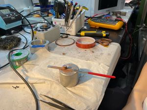
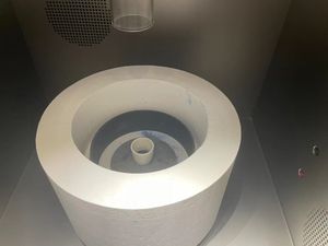
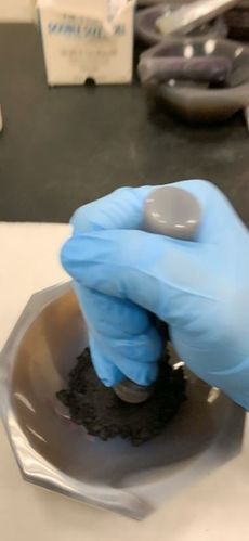
To synthesize La0.95Na0.05MnO3, we use solid-state Microwave Synthesis due to its advantages in short reaction time, low energy consumption and clean reactions. We first take the La2O3, Na2CO3 and Mn2O3 in correct molecular ratio, grind and mix them together, then put the powder into microwave furnace for heating. The temperature is raised to the desired temperature in 20 min with a fixed MW power and the powder is maintained at the final temperature for 30 min for reactions to complete and then the power is switched off. The samples cool to room temperature in 1 hour. After that, the powder was grinded again and the process was repeated for the 2nd time for homogenization. Finally, we press the powder into pellet and subjected to MW irradiation for the 3rd time. The heating temperature and power we use are 1000 degrees Celsius and 1000 Watts. The resistivity of this sample measured by four probes method is about 0.5 Ohm * centimeter.
Experiment Set up
The measuring circuit consists of a detecting coil, a compensating coil with equal turns of copper wire and a primary coil. The primary coil is connected to the Lock-in Amplifier output. An ac current flows through primary coil and gives rise to magnetic field. The detecting coil and the compensating coil are connected to Lock-in Amplifier input so that we can measure the voltage. The compensating coil is used to compensate the voltage in detecting coil without samples. We connect the detecting coil to one port(A) in Lock-in Amplifier and compensating coil in another port(B). The resultant voltage is the difference between two coils which is the voltage induced by the sample. Of course, the sample is placed in the middle of detecting coil and the sample length is short compare to the length between detecting coil and compensating coil so that the Eddy current in the sample has little effect on the compensating coil. In literature, secondary coil is adjusted by position and voltage offset so that voltage without sample is zero. The combination of detecting coil and compensating coil in our set up is analogous to the secondary coil used in literature.
Figure 4 shows the schematic of coils set up. For method one, a and c contact points are connected to port A and b and c points are connected to port B for balancing voltage. For method 2, only a and c contact points are used to be connected with voltmeter measuring root mean square voltage. d and e points are for ac current in.
Figure 5 shows our coils and different terminals. Two terminals on the right are the positive and negative terminals for primary coil. The magnetic field induced by this coil is calculated to be 14.073 * I Oe which I is the applied current controlled by the Lock-in Amplifier. There are three terminals on the left. We connect upper two to for the detecting coil and lower two for the compensating coil. They are connected to different input ports in Lock-in Amplifier. We put tissues in the bottle so that the sample lies in the range of detecting coil
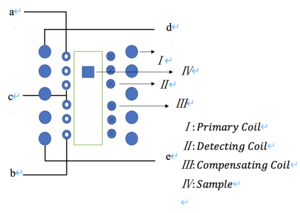
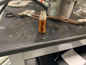
Figure 6 shows the coils connected to wires and Figure 7 shows how they are connected to SR830 Lock-in Amplifier
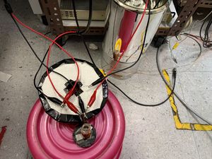
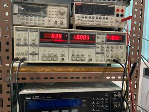
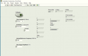
Figure 8 shows the panel of the Labview program we built and Figure 9 is the source code. First, We do one measurement without samples, the program will give us some x, y and theta values. Ideally, the theta value would be 0 because we have the compensating coil. But in reality, the coils are not perfect so that we need to calibrate the system to cancel the phase. The calibration is done by giving some offsets so that theta becomes 0. This is automatically done when we choose the "calibrate" option in the program for the first measurement. Then we insert our samples and measure with calibrate option off. The "x from sample" and "y from sample" in the program will give us the final results which correspond to real and imaginary part of the EMF induced.

Data Analysis
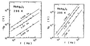
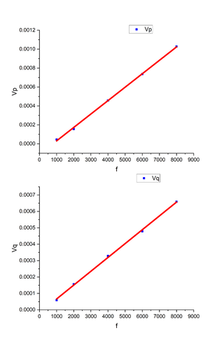
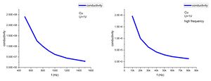
We first measure the copper rod with diameter of 6mm under low frequency range and high frequency range separately both with 1V AC current. From the equations we present in Introduction, we can observe that the real part of the voltage has linear relationship with AC current frequency while the imaginary part has quadratic relationship. However, both Figure 10 (From literature) and Figure 11 (Our measured values) do not show the quadratic dependence of frequency in imaginary response. Instead both Vp and Vq (Figure 10) shows a linear variation with respect to frequency as well as Figure 11 which we suppose to be the intrinsic frequency dependence of ac conductivity. Literature written by Ishida et al. claims they have quadratic relationship but we clearly cannot see that from the graph they provided. We do not quite understand why this is the case. We consulted Doctors in our lab but they could not provide good explanations either. Also, other literature we found do not provide similar graphs. So we just assumed our Voltage vs. Frequency relation is consistent with the equations and moved on to the conductivity. As a result, the conductivity of Cu rod shown in Figure 12 decreases with the increasing of frequency which shows a similar value with dc conductivity around kHz range. Within kHz range, the dimension of our measured result matches the theoretical conductivity of Cu we found online which is around 107 Siemens/meter. This is acceptable because with high frequency, conductivity changes with respect to skin depth which we will explain more in the following section.
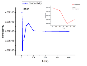
In addition, we measured Teflon which is an insulator for comparison. According to the conductivity vs. frequency graph shown in Figure 13, we can observe alternating positive and negative values in the conductivity with even a singular point. Both Vx and Vy collected from lock-in amplifier shows alternating positive and negative values as well with absolute value in the same magnitude with calibration data which is not acceptable. The magnitude of the alternating data is way off from the theoretical value we found online. As a result, we believe that Teflon induces so weak response to the alternating current that we can hardly measure its ac conductivity. The most oscillations we are getting may not come from the sample itself
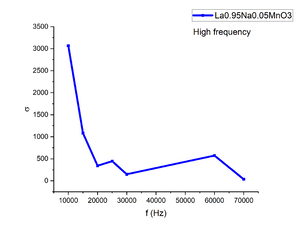
Another sample we measured is La0.95Na0.05MnO3 which is the ferromagnetic insulator at room temperature. The conductivity we measured at tens of kHz range is several orders of magnitude higher than the dc conductivity we measured with the standard four probe method. As it is insulator, the response is weak as well compared to copper rod, which will lead to the inaccuracy of the ac conductivity. Besides, skin depth is much smaller for this sample due to the ferromagnetic nature which will lead to the nonuniform distribution of eddy current in the samples. This will be in contrast with our assumption that eddy current should be uniformly distributed in the sample when we calculate the conductivity. This may be the reason why we get much higher value than dc conductivity.(Figure 14)
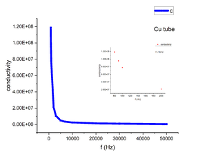
We finally measured the copper tube with the second method mentioned in theory part to compare. We measured the Vrms before and after inserting the sample in to the coils. And we calculated the phase shift from V1 and V2 which finally give the conductivity. Similar result comes in this experiment that ac conductivity shows similar magnitude compare to dc conductivity around kHz range and also shows decreasing relation with respect to frequency.(Figure 15) We may conclude that two methods we found in the literature are both applicable to copper
Conclusion
According to the result we obtain from different materials we measured, it seems that the method we use for ac conductivity has a limitation in non magnetic conductors while ferromagnetic material and insulators are not showing expected results. Although both methods we found are applied only to metals in the paper, this contactless method in principal, according to some other readings we list in Reference, should be applicable to insulators. We did not quite get expected result may due to following reasons:
It comes out that the response of voltage is quite small compared to calibration voltage which indicate the response coming from copper coils not wound well and environment may influence greatly on the final result. To make a improvement, we may better design a support for copper wires to wind them tightly and uniformly and put the whole set up in the vacuum chamber with temperature controller to eliminate the influence of environment.
Skin depth is a very important factor for eddy current distribution in material. For magnets with large permeability, the decreasing of skin depth will lead to inaccuracy in conductivity and no more satisfy the condition that skin depth should be far larger than sample diameters. As well from the formula provided below, we see for high frequency measurement, accurate data are hard to obtain due to the decreasing in skin depth.
Failed to parse (SVG (MathML can be enabled via browser plugin): Invalid response ("Math extension cannot connect to Restbase.") from server "https://wikimedia.org/api/rest_v1/":): {\displaystyle \begin{alignat}{2} \delta & = \frac{1}{\sqrt{\pi\mu_r\mu_0f\sigma}} \end{alignat} }
The set up we made has the configuration with detecting coil surrounding samples which will also lead to inaccuracy in the measurements. The detecting coil around samples is associated to an additional magnetic flux from primary coil irrespective of the presence of the sample. While using tube shape sample, the detecting coils will be more sensitive to magnetic field screened by the tube outside if it's placed in the tube.
In our experiment, the sample we use has lengths only slightly larger than their diameters so that edge effect may contribute a lot here. Further improvements can be made if we use a longer rod which we do not have access to for this time.
Team Members
Chen Guohao, Jiang Luwen
Lab Location
Spintronics and Magnetic Materials Lab
References
- ↑ Ishida, T., Monden, K., & Nakada, I. (1986). Electrodeless method for the measurement of ionic conductivity of RbAg4I5. Review of Scientific Instruments, 57(12), 3081-3084. https://doi.org/10.1063/1.1138995
- ↑ Iñiguez, J., & Raposo, V. (2007). Measurement of conductivity in metals: A simple laboratory experiment on induced currents. European Journal of Physics, 28(6), 1125-1129. https://doi.org/10.1088/0143-0807/28/6/009
3.Bean, C. P., DeBlois, R. W., & Nesbitt, L. B. (1959). Eddy‐Current method for measuring the resistivity of metals. Journal of Applied Physics, 30(12), 1976-1980. https://doi.org/10.1063/1.1735100
4.Crowley, J. D., & Rabson, T. A. (1976). Contactless method of measuring resistivity. Review of Scientific Instruments, 47(6), 712-715. https://doi.org/10.1063/1.1134714
5.Oike, H., Miyagawa, K., Kanoda, K., Taniguchi, H., & Murata, K. (2009). Contactless conductivity measurements on the organic conductor, κ-(ET)4Hg2.89Br8, under pressure. Physica. B, Condensed Matter, 404(3-4), 376-378. https://doi.org/10.1016/j.physb.2008.11.023
6.Kraftmakher, Y. A. (1991). Measurement of electrical resistivity via the effective magnetic susceptibility. Measurement Science & Technology, 2(3), 253-256. https://doi.org/10.1088/0957-0233/2/3/011
7.Bauhofer, W. (1977). Continuous, contactless measurement of the temperature-dependent electrical resistivity of metals. Journal of Physics. E, Scientific Instruments, 10(12), 1212-1214. https://doi.org/10.1088/0022-3735/10/12/003

