Kerr Microscope
"I was led some time ago to think it very likely, that if a beam of plane-polarized light were reflected under proper conditions from the surface of intensely magnetized iron, it would have its plane of polarization turned through a sensible angle in the process of reflection." - John Kerr[1]
Imaging a sample can be done in many ways, depending on the light-matter interaction we are interested in observing. The magneto-optic Kerr effect (MOKE) describes the change in polarization of incident light when it impinges on the surface of a magnetic material. The resultant reflected light can then form an image through focusing optics which provides high contrast between areas of different magnetization.
Through Kerr microscopy, we aim to characterize the relative changes in magnetization across a magnetic sample.
Team members
- Joel Yeo
- Gan Jun Herng
- Sim May Inn
(Feel free to edit this page or email me at joelyeo@u.nus.edu if you would like to join.)
Idea
In this project, we will be aiming to build a basic Kerr microscope using off-the-shelf polarizers, objectives, detectors and laser source. A magnetic sample can be borrowed from a team member's research lab. To increase the field of view, we also plan to incorporate automatic raster scanning of the sample through means of an Arduino-controlled sample stage.
Broadly, our goals are:
- Build an imaging setup
- Image a magnetic sample
- Automate scanning of sample
Overview
This section contains a bird's eye view of our experimental time line. We began the experiment in week 5 of the semester and ended in week 13. In our attempt to observe the Magneto-Optic Kerr effect, we tinkered with two different optical setups. Setup 1 reflects a beam of linearly polarizer light off a magnetic sample which we then pass through an analyzer and capture on our CCD (webcam). Setup 2 more closely resembles a microscope.
| Week | Milestone |
|---|---|
| 5 | Gathering and Initial Setup |
| 6 | Machining and Setup Design |
| 7 | Angled Setup |
| 8 | - |
| 9 | 2x Mirror Alignment |
| 10 | Microscope Setup with 10x Objective |
| 11 | Lab Magnetic Sample and VFL light source |
| 12 | 60x Objective |
| 13 | Final Experimental Readings |
Theory
Magnetic domains

In magnetic materials, there exists magnetic dipoles wherein their magnetic interactions with each other are called dipolar interactions, the strength of which is related to their separations. Such interactions result in the formation of regions of uniform magnetization, also known as magnetic domains. When multiple magnetic domains are formed, magnetostatic energy in the system decreases as the net magnetization of the system is reduced. Common instances where we can find magnetic domains would be in the random arrangement of magnetic domains on refrigerator magnets, and in specific forms within magnetic recording devices such as magnetic tapes and Video Home System (VHS) tapes. Several domain imaging techniques can be used to observe and study these magnetic domains, and the most inexpensive, time saving, and least intrusive method would be through Magneto-optical Kerr Effect imaging technique.
Magneto-Optical Kerr Effect (MOKE)
Conceived by John Kerr in 1877[3], the magneto-optic Kerr effect (MOKE) describes the rotation of light polarization when reflected from a magnetized surface. MOKE can be further categorized depending on the relative orientations of the reflecting plane to the magnetic field.
Light reflected from a magnetized surface may change both polarization and reflected intensity. This comes about because the magneto-optic material has an anisotropic permittivity, meaning that the permittivity depends on the direction. The permittivity affects speed of light in a material. Therefore, light entering the material would be slowed by different amounts depending on its polarization.

MOKE microscopy
Interaction between an incident light and the magnetization of a magnetic sample causes a change in polarization state of the incident light. MOKE microscopy makes use of the fact that varying magnetizations corresponding to different magnetic domains on the sample gives rise to different degrees of incident light polarization. By detecting and imaging these reflected or transmitted interacted light, an image of magnetic domains with varying intensities can be observed, thereby allowing for domain imaging to be conducted. Basic components of a MOKE microscope includes, firstly the light source lamp, which is fed through a microscope array with polarizers and analyzers onto a sample with an accompanying magnet to change the applied magnetic field, and the resultant light is collected in a camera. Subsequent image processing is required to elucidate weak changes in contrasts.

MOKE imaging modes
Experiments involving the different MOKE orientations are typically carried out in the following manner, in accordance to data acquisition conditions and the sampled materials' suitability.
- Polar MOKE -- Near normal incidence to avoid Kerr rotation.
- Longitudinal MOKE -- Incidence at an angle to surface, parallel to field. Linearly polarized light becomes elliptically polarized. The change in polarization is directly proportional to .
- Transverse MOKE -- Incidence at an angle to surface, perpendicular to field. This affects reflectivity . Viewed from the source, if points to the right of the incident plane, the Kerr vector adds to the Fresnel amplitude vector and the intensity of the reflected light is . If it points to the left, it is .


Experimental Setup
This section details the two main iterations of our experimental setup - the angled setup and the microscope setup.
Location: S11-02-04
Equipment:
- Power Supply
- Red LED
- Red Laser Diode
- Red Laser Pen (Visual Fault Locator)
- Pinhole Aperture
- Plano-convex lens (100mm, 150mm, 300mm)
- Translation stage x2
- Sheet Polarizer x2
- CCD Array (Webcam)
- Magnetic samples
- Steel sheet wound with copper wire
- Magnetic tape from floppy disk & cassette tape
- Magnetic film on Si/SiO2 substrate (lab sample)
Setup 1: Angled Setup
-
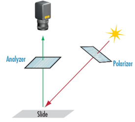 Angled Setup Schematic. A polarized light source is reflected off our sample at an angle, passed through an analyzer and finally recorded on our CCD array.
 -
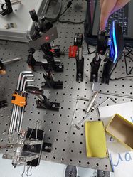 Setup 1. The laser pointer is mounted on an acrylic stand shown in bottom left of image.


As a first observation of the MOKE, we utilized a basic setup that reflected a linearly polarized light source off our sample - an electromagnet that consists of a steel sheet wrapped with copper wire. The light source is an off-the-shelf red laser pointer. The reflected beam is focused by a plano-convex lens and passed through an analyzer before it is finally captured on our CCD array (webcam). The open source video capture software OBS was used to display the captured image.
The intention with this setup is that if we align the axes of the polarizer and analyzer, the beam would be completely extinguished for a non-magnetic sample. Then, regardless of which of the three MOKE effects were at play, a magnetic sample would alter the polarization of the reflected beam, causing it to only be partially extinguished by the analyzer. In practice, since we are working with non-ideal polarizers that have high extinction ratios (but not 100%), the image of a non-magnetic sample would have been used as a baseline for comparison with a magnetic sample. By exporting image captures from the OBS software and isolating the pixel intensities, a study could have been done by taking the differences in pixel intensities between the two images.
Alas, while the experimental setup was simple, the greatest stumbling block proved to be the very first step - capturing an image. Aligning all the optical components proved to be challenging and time consuming, particularly when shifting the webcam back and forth in an attempt to focus the image since this meant unscrewing the base, adjusting the position of the webcam, and tilting the base at an angle to fit a screw back into the optical table. On the suggestion of Prof. Christian, we cobbled together a crude z-translation stage which used two additional base holders to 'lock' onto the base of the webcam from either side and allow movement only along the optical axis. This did not solve the alignment issue directly, but it did allow us to identify another problem that we ought to tackle first.
The laser pointer casing was slightly bulbous toward the front end. This meant that when it was mounted onto the acrylic holder (see image), it was tilted up slightly, and thus the plane in which the light beam travelled was not parallel to the optical table but tilted upward. Consequently, for every shift of our webcam along the z-axis, a corresponding change in height would have to be made. This made the alignment procedure particularly tedious. At this juncture, a decision was made to modify the light source before proceeding with imaging.
Setup 1.1: Double Mirror Alignment

This change to the setup was made in response to alignment woes.
Main Change:
- Added two mirrors attached to adjustable mounts.
Other Minor Changes:
- Added a second lens to focus an image onto the CCD array, rather than the beam itself.
- Swapped to a sample with a smoother surface - the magnetic tape of a floppy disk - to reduce diffuse reflection.
- Swapped to a 650nm laser diode (Datasheet) as the red laser pointer produced a rather 'dirty' beam with various artifacts.
The usage of the mirrors for alignment is as follows:
-
 Pinhole near.
 -
 Pinhole far.


- Place a pinhole aperture near the second mirror and turn the knobs on the first mirror to adjust the pitch and yaw until the laser beam is centered on the pinhole.
- Swap the pinhole to a location farther down the beam path. Tune the knobs on the second mirror until the beam is centered.
- Repeat steps 1 and 2, continuously swapping the pinhole between the near and far locations until the beam passes through the pinhole at both locations.
Result: Still unable to obtain a good image of our sample. Our beam does not cover a large enough region of our CCD array and the majority of what we are imaging is likely from ambient light sources. Alignment also proves difficult as it is sometimes hard to discern the light that originates from our light source. At this juncture, a decision was made to modify the rest of the optical setup to increase magnification.
Setup 2: Microscope Setup
-
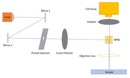 Schematic of microscope setup. The two mirrors facilitate beam alignment.
 -
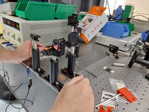
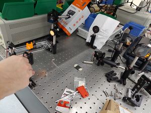
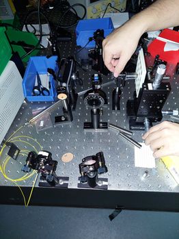 Microscope setup, sans pinhole after Mirror 2. The light source is at the bottom left.


This change was made in an effort to increase the magnification of our imaging setup.
Main change:
- Revamped optical setup to resemble that of a microscope.
Other minor changes:
- Switched light source once more to a laser pen (aka Visual Fault Locator) coupled to a single mode fiber for an even cleaner light source.
- Swapped to a lab prepared magnetic sample.
- Added micrometer screw translation stage for sample.
When working with microscope objectives, it is important to be aware of the tube length, which is the distance between the objective and the image produced by the objective. We used an objective that was manufactured according to the DIN standard, which specifies a 160mm tube length. Hence, we positioned our CCD array 160mm away from the objective to capture the image. If working with an RMS objective, the tube length is 170mm instead[4]. A second parameter that must be kept in mind is the working distance, which is the distance that the sample must be placed in front of the objective. For the 10x and 60x objective, these are 1.5mm and 0.15mm respectively[5][6]. Hence, when using the 60x objective, the sample is practically kissing the objective.
The use of a micrometer screw translation stage allowed for finer control over the position of our sample to a precision of microns (5 micron contribution from both ends of the measurement).

To test the iterated setups, two main samples were used, in addition to a series of permanent magnets. The first, a standard empty Si/SiO2 substrate as a control sample. The second, a magnetic sample whose external field will be controlled by a magnet stack. This magnet stack was attached to a second translation stage and held close to our samples. The external field strength affecting our sample could then be controlled by moving the magnet closer or farther from our samples, and the distance travelled can be read off from the micrometer screw gauge. In terms of imaging, if stripe domains are the brighter features, the expected overall intensity garnered from the setup will decrease as the field increases, and vice versa if the stripe domains turn out to be the darker features.
-
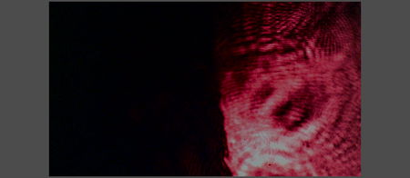 OBS screen capture - Imaging the edge of our sample with a 60x microscope objective.

In this final iteration, we are happy to report that imaging was a success. We were able to observe the presence of defects and dirt particles on the surface of our samples. And as a quick estimation of the size of our imaging region, we honed in on the edge of our magnetic sample and tuned the micrometer stage such that the edge moved from end of the screen to the other. The distance moved by the edge can then be read off from the screw gauge. In this manner, we found the 10x objective to give an image size 370 microns across and the 60x objective to give an image size 60 microns approximately (with the associated 10 microns uncertainty).
Results and Analysis
Series of permanent magnets

In this project, we were provided with numerous tiny neodymium disc magnets. We stacked these magnets to produce a larger magnet with a stronger overall magnetic field. The geometry of the stack also resembled more closely a bar magnet, which produces a reasonably uniform magnetic field at its tips. After dismantling the setup, the magnet stack was removed and brought to a lab to check out the external field with a Hall meter. The maximum field at the surface of the magnet, in contact with the back of the sample was measured to be -0.473 T. By varying the separation between the magnet stack surface and the probe from 0 to 40 mm, we measured the external field to vary from -0.473 T to -0.005 T.
Polarization dependent intensity changes
In commercial MOKE microscopy systems, the initial measurement steps often includes locating the ideal polarization angle which works with the specific sample. In light of this, we first performed polarization angle dependent intensity studies by removing the external field provided by the magnet stack. Doing so, we could determine which polarization angle (1) works best with our setup and camera, as well as (2) gives us decent signal to be able to observe changes in intensity. The former ensures that the camera is operational and not oversaturated during the data collection process. After obtaining these insights on the selection of polarizer angle, we proceeded to take measurements at the determined angle as well as the neighbourhood of this angle to obtain information about polarization dependent intensity changes.
Field dependent intensity changes
Since Kerr imaging is based on the non-linear response of the sample with respect to the incident light intensity, we considered two alternative lighting configurations -- one in which the laser beam was collimated, and another in which the laser beam was focused onto the sample plane to maximize the incident intensity. The CCD was connected to a computer, and the images were captured on the Open Broadcaster Software (OBS) program. We turned off the auto-exposure settings in OBS to ensure consistent imaging conditions across all our measurements. Each measurement was then exported as a .png file and further processed in Python as uint8 images.
-
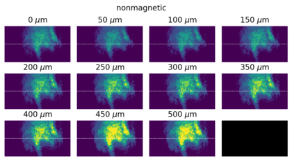 Measured images from non-magnetic sample illuminated by a collimated beam. The white, dashed line denotes the line profile we analyzed.
 -
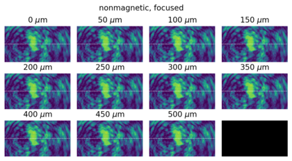 Measured images from non-magnetic sample illuminated by a focused beam. The white, dashed line denotes the line profile we analyzed.
 -
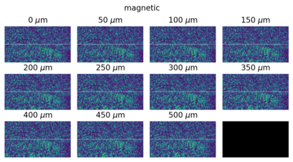 Measured images from magnetic sample illuminated by a collimated beam. The white, dashed line denotes the line profile we analyzed.
 -
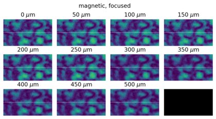 Measured images from magnetic sample illuminated by a focused beam. The white, dashed line denotes the line profile we analyzed.


The four figures above depict the raw measurements captured by our Kerr microscopy setup for the four different cases corresponding to the type of sample we were imaging as well as the lighting configuration. Yellow depicts a higher pixel value (intensity), and blue vice versa. The labeled distance of m above each individual image denotes the estimated separation distance between the bar magnet and the back of the sample. In all cases, the magnification was kept the same. The vastly different features seen between the 4 cases are likely due to different areas of each sample being imaged upon changing the lighting and sample configurations.

-
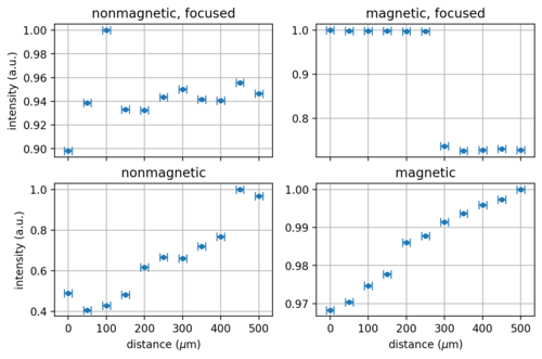 Summed image intensities against sample-magnet distance.

In order to obtain a more quantitative evaluation of whether the Kerr effect is present in our measurements, we summed the pixel intensities in each captured image and plotted the result with respect to the sample-magnet distance (analogous to external magnetic field strength). For a simpler comparison, we also normalized the graphs such that the maximum intensity is 1. The horizontal error bars are 10 m, corresponding to the precision of our micrometer screw gauge. Interestingly, we observed a rather consistent intensity across all sample-magnet distances for the focused laser beam, as opposed to the increasing trend for the collimated laser beam case. The sudden jump of intensity from 1 to ~0.7 in the top right quadrant is likely due to an accidental change in our setup apparatus whilst we were moving the sample stage from 250 m to 300 m.


The non-increasing trend observed in the top two quadrants is consistent with what we expect from theory. For a non-magnetic sample, the MOKE should not be present as silicon on its own is not magnetic, and therefore should not result in a change in light polarization. Based on the magnetic field strength as a function of distance previously measured, we believe that the field strength experienced by the magnetic sample even at the furthest distance of 500 m is strong enough to saturate the magnetization of the sample. Therefore, we are unable to observe any changes in the intensity of light for this range of distances. Due to time limitations, we were unable to go back to the lab to collect more data for distances further away where the field strength should be small enough for us to theoretically recover the hysteresis curve we expect from MOKE.
For the increasing trends seen in the bottom two quadrants, we suspect that these are evidence of systematic errors during our measurement process because they are inconsistent with what we expect to observe from our simple setup. For the non-magnetic material illuminated with collimated light, it should also result in an unchanged intensity regardless of the external magnetic field. On the other hand for the magnetic sample, the effect of MOKE should be much lesser for collimated illumination as compared to the previously focused illumination due to a lower incident intensity on the sample. Hence, if the focused illumination for the magnetic sample shows a flat trend due to saturation, we should also expect a flat trend for the bottom right quadrant as opposed to the increasing trend we see.
-
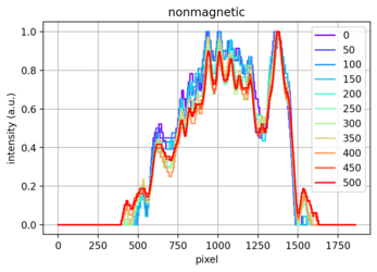 Line profiles across row 500 of each captured image from the non-magnetic, collimated dataset.
 -
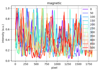 Line profiles across row 500 of each captured image from the magnetic, collimated dataset.
 -
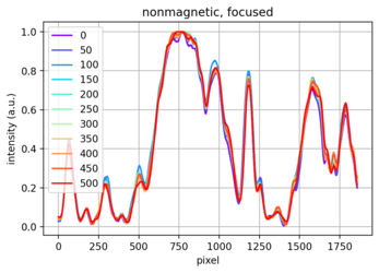 Line profiles across row 500 of each captured image from the non-magnetic, focused dataset. Here, the line profile features are largely consistent across all sample-magnet distances.


A possible explanation for these increasing trends could be due to the fact that our samples happened to be drifting during the process of collecting these set of measurements. During our experiments, we would sometimes observe that the sample is slowly getting dislodged from its mount as we were only using blue-tacs to hold the sample vertically in place during our measurements. To verify if this could be true, we zoomed into the line profiles of a specific row (since the sample will likely drop down due to gravity) in each of our images to see if we are able to observe any drift in the features. The line profiles are further normalized to have a maximum value of 1 for a fair comparison. The above, left two figures do appear to indicate some form of drifting, as we see that the features for different sample-magnet distances are changing despite normalizing the intensities. For comparison, we also included the line profile for the non-magnetic sample with focused illumination on the right, and we clearly see that the features of each line profile for all sample-magnet distances are largely consistent with negligible changes.
Improvements and Reflections
This section contains our reflections on the experiment and some thoughts on how we, or anyone else wishing to reproduce and improve, could have done better.
Making our own experimental parts - For our group members, it was the first time soldering, cutting, deburring and so forth. We tinkered with our light source and also made our own magnetic sample. This was fresh and fun, although surprisingly time consuming.
Aligning - Realigning our optical setup each time we modified our light source or sample was the most costly in terms of experimental runtime. This got better over time as we got more familiar with our setup and had a better feel of how to tune certain parts. The addition of the double mirrors for beam alignment as well as an xyz-translation stage for holding our sample also streamlined the alignment process. In hindsight however, we should have taken more time to consider each change we wished to make before actually implementing it.
Managing the external fields from magnets - The first improvement we would like to implement would be to collect data from the magnetic sample at lower external magnetic fields, where the magnets are much further away from the sample surface. As the sample saturates at about 0.1 T, we would not be able to observe the changes in domains at fields higher than 0.1 T. It would be great for us to have a Hall meter on hand such that we could measure the external field provided by the series of magnets at the varying separation from the sample.
Lock-in-amplifier - The data that we have collected thus far may indicate the weakness of the Kerr effect, such that no to low observable changes were captured by the camera. When low signals are concerned, lock-in-amplifiers come to mind. We could implement a lock-in-amplifier in the setup, possibly with a chopper as well to send pulsed signals to the sample. With this, even minute changes in intensity could be detected. However, instead of MOKE microscope, our setup would be more of a spectroscope!
Less monochromatic/coherent light source - Using a red laser gave unwanted interference patterns when illuminating our light source. This made it difficult to discern MOKE effects. Using the laser diode (not the laser pen), we attempted a workaround where we reduced the voltage supply to just below the lasing threshold. In this regime, the diode cannot lase and behaves closer to an LED with a broader bandwidth. However, this also reduced the intensity of the light hitting the sample to the point where we could barely see it. If tasked to redo the experiment, we would put more care into sourcing an appropriate light source for our needs.
Surface conditions - The samples used did not have perfectly smooth surfaces which could have contributed to the scattering observed. For instance, the Si/SiO2 empty substrate had scratches on it, likely due to inadequate handling, and extra efforts had to be implemented to avoid such regions. Better handling and care for the surfaces would be recommended as MOKE is a surface related technique.
Summary
Goals (as at top of page):
- Build an imaging setup (eg. Microscope)
- Image a magnetic sample
- Automate scanning of the sample
In view of our stated goals, we were successful in the first and halfway towards accomplishing the second. We built a working 10x/60x microscope with a sample stage that could be translated with a precision of ten microns. However, we could not directly observe the magnetization characteristics of our sample on either the computer screen or even after post-processing of our images. Due to a lack of time and also the subpar performance of our Kerr microscope, we decided to forgo the automated scanning portion as we were unable to obtain decent static Kerr images in the first place.
APPENDIX: Lab Session Logs
10 Feb 2022

Hunted down the required parts. We used the diagram from NaBiS from Politechnico di Milano’s physics department as our guide[7].
Linear polarizer was found, but extremely dirty. First rinsed with water than finished cleaning with isopropanol (IPA). IPA available in S11-02-04 room cupboard. Discussed some other things between us and with TAs:
- Stage requires mm precision

We only used the two knobs on the right hand side. First turn the voltage up slightly to set a limiting voltage, then slowly turn on the current till the LED turns on. Observation shows LED tends to turn on at about 2V. The positive end (red) should be connected to the positive (anode) side of the LED. This can be seen as the longer leg of the LED.
15 Feb 2022
From the info on the NaBiS page, we may need to characterise the material in all three MOKE orientations to get a full 3D image. But we’ll think about that later.
Today was more parts gathering, a little machining to make the parts that we need.
Magnetic material - Got a bunch of steel sheets from CK, and some copper wire to wrap around it like a mini solenoid. The sheets are a soft magnetic material ( = 5000 − 7000 according to CK) and will be magnetised when a current runs through. CK suggested we set it up so we can change the direction of the magnetic field by switching ??? (not exactly sure, will need to figure out later), and not manually moving the sample. Might be easier down the road.
The steel sheet was cut with some steel cutting scissors, and de-burred with sandpaper. The copper wires had to be stripped for connection. This was done with some Stanley blades and polished with some sandpaper. Not the cleanest, but as long as we get a current it’s fine.
18 Mar 2022
Field of view provided by the webcam was too wide in comparison to the laser spot. Ideally, the image should be less than the diameter of the laser spot. A few methods were proposed in response to this:
- If we were unable to see the actual area, we should minimally be able to see a change in intensity of the imaged spot, with and without a magnetic sample. However, we were not able to observe such variation in intensity, probably due to the small size of the area of interest, and the weak signals we were receiving.
- Attempted to block out all ambient light, and isolate only the signals from the laser spot, but again, we were not able to observe any obvious variation in intensity.
- Propose the use of a beam expander before the camera - was not implemented yet.
- Remove the blue LED about the camera which was initially there for simply aesthetics. Soldering was utilised to remove the relevant circuits and parts from the board.
- Removed the lens in the camera, which causes the wide view.
Next: to test if LED and lens removal helped ease the situation.
29 Mar 2022
- Alignment attempts and measuring of imaged frame size.
- Attempt to image small features such as the anticounterfeit print on a $2 bank note.
5 Apr 2022
- The polarizer sheet has too many scratches and marks to work with, to switch it out to another better quality polarizer.
- To change light source to a fibre coupled laser source instead and check out how it fairs in comparison.
8 Apr 2022
- Try to misalign beam to prevent interference or whatever is happening at NPBS interface
- Switch to LED light source. Might be challenging to couple beam into fiber, but should get rid of interference fringes
- Illuminate at angle rather than on-axis. Might be hard to aim beam since sample is so close to objective. This might help reduce any interference between incoming and reflected beam
13 Apr 2022
Final alignment and field dependent imaging session.
References
- ↑ J.Kerr, Philosophical Magazine 3 (1877) p.312.
- ↑ Rudolf Schafer - Magneto-optical microscopy and its application..
- ↑ P.Weinberger writes about Kerr's famous communications to the Philosophical Magazine - Wayback Machine.
- ↑ DIN Standard Microscope Objective Lenses - Microscope World.
- ↑ 10x Objective - Edmund Optics
- ↑ 60x Objective - Edmund Optics
- ↑ Kerr microscope schematic – NaBiS