Orbits of the Galilean Moons

Galileo Galilei’s discovery of celestial bodies that orbit something other than the Earth marked the beginning of the end of the geocentric model of the universe. In this project, we will perform the same observations on those moons as Galileo did 400 years ago.
Team Members
- A0168128Y Matthew Wee
Objectives
- To observe the planet Jupiter and its four largest moons—Io, Europa, Ganymede, and Callisto
- To measure the orbital parameters of those four moons, such as orbital period and radius
- To explore the orbital resonances of the inner three of those moons—Io, Europa, and Ganymede
- To verify Kepler’s Third Law
- To assess the viability of consumer equipment in performing precise scientific measurements
History

Jupiter is a planet that was known to the ancients as it is the fourth brightest object in the sky behind the Sun, the Moon, and Venus, and is visible to the naked eye. In 1609, astronomer Galileo Galilei made improvements to his telescope, which was the best in the world at the time. With the telescope, over the course of several weeks, he observed four “stars” moving in a line around Jupiter and was persuaded after just four days of observations that they were not stationary stars but instead objects orbiting the planet Jupiter. German astronomer Simon Marius also made this discovery independently and at the same time, but he is lesser known because he published his observations only after Galileo did. He had the privilege, however, of having his names of these moons (Io, Europa, Ganymede, Callisto) be widely accepted, much to Galileo's dismay.
The discovery that there exist objects that do not orbit the Earth, along with several other breakthroughs, was the cornerstone of the Copernican Revolution, which was the transition from the geocentric to the heliocentric model, with the Sun instead of the Earth at the center of the universe.
Since then, astronomers have discovered a total of 80 moons that orbit Jupiter, 23 of which have no official names.
Background
The four Galilean moons, in increasing order of orbital radius, are Io, Europa, Ganymede, and Callisto, of which, Io, Callisto, and Ganymede are larger than the Earth's Moon in both mass and diameter. Ganymede is even larger than the planet Mercury. Because of their size, they can be observed from Earth with a small telescope or even a pair of powerful binoculars.
The main challenge faced when trying to observe these moons is the sheer brightness of Jupiter relative to the dim moons, and their small angular separation from Jupiter. This is especially true for the innermost moons Io and Europa.
Apparatus

No specialized equipment was used in this experiment to make observations of the planet and its moons.
- Canon EOS 60D DSLR[1]
- APS-C sensor (1.6× crop)
- Pixel size 4.31µm
- Sigma 150–600mm f/5–6.3[2]
- Lens diameter 95mm
- Field of view: 16.4º–4.1º (effective 10.2º–2.6º)
- Low-end consumer tripod
- Spirit level
- Remote shutter
Exposure Settings
- Manual
- Focal length: 600mm (effective 960mm)
- 1/15s exposure
- f/6.3 aperture
- ISO 3200 sensitivity
- Manual focus
- Image stabilization off
The exposure time cannot be set for too long as motion blur due to the Earth's rotation will be visible in the image.
Data


Procedure
A series of observations were performed with the telephoto lens mounted on the camera. Weather permitting, exposures were taken every day within an hour of sunset for two and a half calendar weeks from 31 January 2022 to 17 February 2022.
At the time of these observations, Earth's motion around the Sun (and to a lesser extent, Jupiter's as well) caused the apparent position of Jupiter in the sky to drift closer to the sun every day, forcing observations to occur closer and closer to sunset. The last observation on 17 February was taken at 7:59 PM, when the sun had barely set and the sky was still relatively bright (compared to the dim moons). It was decided that no more observations could be taken thereafter.
The moons in the captured images were identified using Stellarium or Night Sky.
By inspecting the moons and their positions relative to Jupiter in the captured images, their apparent angular separation can be determined for every observation. The data are presented in the table below.
Raw Data
| Observation | Angular distance between moon and center of Jupiter (arbitrary units) | |||
|---|---|---|---|---|
| Io | Europa | Ganymede | Callisto | |
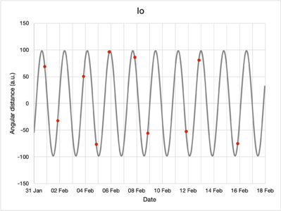
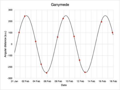
| 2022-01-31 | 68.9 | occultation | 102.7 | -254.2 |
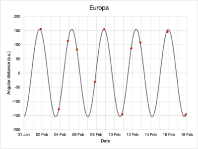
| 2022-02-01 | -32.2 | 155.4 | 245.7 | -371.0 |
| 2022-02-02 | no data collected | |||
| 2022-02-03 | 50.6 | -127.9 | 23.8 | -437.9 |
| 2022-02-04 | -76.3 | 113.8 | -175.9 | -392.3 |
| 2022-02-05 | 96.4 | 83.2 | -251.8 | -284.4 |
| 2022-02-06 | no data collected | |||
| 2022-02-07 | 86.2 | -31.0 | 62.2 | 25.5 |
| 2022-02-08 | -55.7 | 154.5 | 224.8 | 183.0 |
| 2022-02-09 | no data collected | |||
| 2022-02-10 | occultation | -145.8 | 68.0 | 405.6 |
| 2022-02-11 | -52.4 | 87.2 | -140.1 | 437.5 |
| 2022-02-12 | 81.0 | 108.1 | -246.5 | 408.5 |
| 2022-02-13 | no data collected | |||
| 2022-02-14 | no data collected | |||
| 2022-02-15 | -75.2 | 145.8 | 195.9 | 40.0 |
| 2022-02-16 | no data collected | |||
| 2022-02-17 | transit | -147.2 | 101.8 | -252.2 |
When a moon is occulted by Jupiter, it is not visible and its position cannot be determined with precision. Similarly, during a transit, Jupiter outshines the moon and its precise position also cannot be determined. Either way, that day's observations are not included in that moon's dataset.
Inclement weather and other circumstances have also prevented data collection on certain days as indicated.
While angular distances do not have negative values, the signs represent whether that moon has a greater or lower elevation in the sky compared to Jupiter; this helps differentiate in which part of their orbits the moons are for the purposes of modeling.
Modeling

Center: apparent positions as viewed by a distant observer from Earth
Right: the apparent position plotted over time
The equation used to model the motion of the moons is

where is the angular displacement between the moon and Jupiter as a function of time Failed to parse (SVG (MathML can be enabled via browser plugin): Invalid response ("Math extension cannot connect to Restbase.") from server "https://wikimedia.org/api/rest_v1/":): {\displaystyle t} , Failed to parse (SVG (MathML can be enabled via browser plugin): Invalid response ("Math extension cannot connect to Restbase.") from server "https://wikimedia.org/api/rest_v1/":): {\displaystyle a} is the amplitude of the moon's oscillation about Jupiter, proportional to its semi-major axis, Failed to parse (SVG (MathML can be enabled via browser plugin): Invalid response ("Math extension cannot connect to Restbase.") from server "https://wikimedia.org/api/rest_v1/":): {\displaystyle T} is the period of the orbit, and Failed to parse (SVG (MathML can be enabled via browser plugin): Invalid response ("Math extension cannot connect to Restbase.") from server "https://wikimedia.org/api/rest_v1/":): {\displaystyle \phi} is the phase of the orbit.

A simple sinusoid is used to the model the moons' motions. By projecting uniform circular motion unto the plane of the sky, a pure sinusoidal wave would be obtained. In order to use this model, the following assumptions must be made:
- The inclination of the moons' orbits are 90º.
- The orbital paths of the moons are circular, and as a result
- the moons have constant angular velocity.
- the moons maintain a constant distance from Jupiter.
- The distance between the Earth and the Jovian system remains constant.
The validity of these assumptions will be discussed later.
Amplitude Failed to parse (SVG (MathML can be enabled via browser plugin): Invalid response ("Math extension cannot connect to Restbase.") from server "https://wikimedia.org/api/rest_v1/":): {\displaystyle a} is expressed in units of pixels, and is approximately proportional to angular distance. Time Failed to parse (SVG (MathML can be enabled via browser plugin): Invalid response ("Math extension cannot connect to Restbase.") from server "https://wikimedia.org/api/rest_v1/":): {\displaystyle t} is expressed in units of calendar days from the midnight starting 31 January 2022, Singapore civil time. For example, if an observation is made on 31 January 6:00 PM, . Period Failed to parse (SVG (MathML can be enabled via browser plugin): Invalid response ("Math extension cannot connect to Restbase.") from server "https://wikimedia.org/api/rest_v1/":): {\displaystyle T} is also expressed in units of days (d). The phase Failed to parse (SVG (MathML can be enabled via browser plugin): Invalid response ("Math extension cannot connect to Restbase.") from server "https://wikimedia.org/api/rest_v1/":): {\displaystyle \phi} serves only to fit the sinusoidal function to the data and is not physically meaningful in this analysis.

Results
The following analyses were done in Wolfram Mathematica and Microsoft Excel.
Fitted Parameters
Using the Mathematica FindFit function, the collected data were fitted to the model, obtaining the following parameters, rounded to four significant figures:
| Satellite | Amplitude Failed to parse (SVG (MathML can be enabled via browser plugin): Invalid response ("Math extension cannot connect to Restbase.") from server "https://wikimedia.org/api/rest_v1/":): {\textstyle a} (a.u.) |
Period Failed to parse (SVG (MathML can be enabled via browser plugin): Invalid response ("Math extension cannot connect to Restbase.") from server "https://wikimedia.org/api/rest_v1/":): {\displaystyle T} (d) |
Phase Failed to parse (SVG (MathML can be enabled via browser plugin): Invalid response ("Math extension cannot connect to Restbase.") from server "https://wikimedia.org/api/rest_v1/":): {\displaystyle \phi} (rad) |
|---|---|---|---|
| Io | 98.38 | 1.770 | 5.701 |
| Europa | 154.7 | 3.555 | 4.807 |
| Ganymede | 249.3 | 7.196 | 5.975 |
| Callisto | 441.7 | 16.92 | 3.433 |
Angular distance is expressed in arbitrary units (a.u.), not astronomical units (AU).
Plots
- Plots of Observations and Fitted Models
-
-
-
-
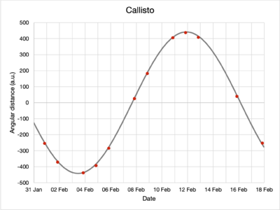


All dates and times are expressed in Singapore standard time (UTC+08:00).
The red dots plot the observations made while the grey lines denote the fitted model. Note the differences in vertical axis scaling.
Comparisons with Literature Values
Visually, from the plots, the model of the moons' motions seem to fit the observed data well.
Orbital Period
| Satellite | Observed Period (d) |
Actual Period (d)[3] |
Discrepancy |
|---|---|---|---|
| Io | 1.770 | 1.769 | 0.063% |
| Europa | 3.555 | 3.551 | 0.104% |
| Ganymede | 7.196 | 7.155 | 0.570% |
| Callisto | 16.92 | 16.69 | 1.407% |
The discrepancies between the empirical data and the literature values are small but increase with increasing period.
Orbital Radii
Because the distance to Jupiter is not known in this exercise, the actual orbital radius (in kilometers) of each moon cannot be inferred from the observations alone. Instead the ratios of the orbital radii of the three outer moons to Io are taken and compared to the literature values.
| Satellite | Observed Amplitude (a.u.) |
Observed Ratio (relative to Io) |
Actual Semi-major Axis (km)[3] |
Actual Ratio (relative to Io) |
Discrepancy |
|---|---|---|---|---|---|
| Io | 98.38 | 1 | 422 000 | 1 | - |
| Europa | 154.7 | 1.573 | 671 000 | 1.590 | 1.079% |
| Ganymede | 249.3 | 2.534 | 1 070 000 | 2.536 | 0.075% |
| Callisto | 441.7 | 4.490 | 1 883 000 | 4.462 | 0.625% |
Again, the discrepancies between the empirical data and the literature values are small.
Orbital Resonance
By expressing the orbital periods in multiples of the period of Io, the orbital resonance phenomenon between Io, Europa, and Ganymede can be identified.
| Satellite | Observed Period (relative to Io) |
Actual Period (relative to Io) |
Discrepancy |
|---|---|---|---|
| Io | 1 | 1 | - |
| Europa | 2.008 | 2.007 | 0.041% |
| Ganymede | 4.065 | 4.045 | 0.506% |
| Callisto | 9.561 | 9.434 | 1.343% |
The relative periods between the three innermost moons are small integer multiples of each other—characteristic of bodies in orbital resonance. The oscillating gravitational influence they experience between themselves is a stable interaction that ensures their relative positions maintain over time. Callisto does not seem to participate in this arrangement.
Kepler's Third Law
Kepler's third law of planetary motion, in mathematical terms, reads that for all objects orbiting the same primary massive object,
Failed to parse (SVG (MathML can be enabled via browser plugin): Invalid response ("Math extension cannot connect to Restbase.") from server "https://wikimedia.org/api/rest_v1/":): {\displaystyle T^2\propto a^3}
where Failed to parse (SVG (MathML can be enabled via browser plugin): Invalid response ("Math extension cannot connect to Restbase.") from server "https://wikimedia.org/api/rest_v1/":): {\displaystyle T} is the period of the orbit and is the semi-major axis of the orbit.

Kepler published these laws with the Sun and planets in mind (hence "Kepler's laws of planetary motion"), but they also apply to moons orbiting planets as well.
| Satellite | Observed Amplitude Failed to parse (SVG (MathML can be enabled via browser plugin): Invalid response ("Math extension cannot connect to Restbase.") from server "https://wikimedia.org/api/rest_v1/":): {\displaystyle a} (a.u.) |
Observed Period Failed to parse (SVG (MathML can be enabled via browser plugin): Invalid response ("Math extension cannot connect to Restbase.") from server "https://wikimedia.org/api/rest_v1/":): {\displaystyle T} (d) |
Constant of proportionality Failed to parse (SVG (MathML can be enabled via browser plugin): Invalid response ("Math extension cannot connect to Restbase.") from server "https://wikimedia.org/api/rest_v1/":): {\displaystyle \frac{a^3}{T^2}} |
Discrepancy from Mean |
|---|---|---|---|---|
| Io | 98.38 | 1.770 | 303 900 | 1.539% |
| Europa | 154.7 | 3.555 | 293 300 | 2.022% |
| Ganymede | 249.3 | 7.193 | 299 100 | 0.065% |
| Callisto | 441.7 | 16.92 | 301 000 | 0.547% |
Derivation
By equating Newton's Law of universal gravitation with centripetal acceleration,
Failed to parse (SVG (MathML can be enabled via browser plugin): Invalid response ("Math extension cannot connect to Restbase.") from server "https://wikimedia.org/api/rest_v1/":): {\displaystyle G\frac{Mm}{r^2}=mr\omega^2}
where Failed to parse (SVG (MathML can be enabled via browser plugin): Invalid response ("Math extension cannot connect to Restbase.") from server "https://wikimedia.org/api/rest_v1/":): {\displaystyle G} is the gravitational constant, Failed to parse (SVG (MathML can be enabled via browser plugin): Invalid response ("Math extension cannot connect to Restbase.") from server "https://wikimedia.org/api/rest_v1/":): {\displaystyle M} is the mass of Jupiter, Failed to parse (SVG (MathML can be enabled via browser plugin): Invalid response ("Math extension cannot connect to Restbase.") from server "https://wikimedia.org/api/rest_v1/":): {\displaystyle m} is the mass of the moon, Failed to parse (SVG (MathML can be enabled via browser plugin): Invalid response ("Math extension cannot connect to Restbase.") from server "https://wikimedia.org/api/rest_v1/":): {\displaystyle r} is the radius of the moon's orbit, and Failed to parse (SVG (MathML can be enabled via browser plugin): Invalid response ("Math extension cannot connect to Restbase.") from server "https://wikimedia.org/api/rest_v1/":): {\textstyle \omega=\frac{2\pi}T} is the angular velocity of the moon.

By expressing angular velocity in terms of orbital period and rearranging,


Failed to parse (SVG (MathML can be enabled via browser plugin): Invalid response ("Math extension cannot connect to Restbase.") from server "https://wikimedia.org/api/rest_v1/":): {\displaystyle \begin{align}G\frac{Mm}{r^2}&=mr\left(\frac{2\pi}T\right)^2\\T^2&=\left(\frac{4\pi^2}{GM}\right)r^3\\T^2&\propto r^3\end{align}}
So proving Kepler's third law. Additionally, by linearizing the equation,
Failed to parse (SVG (MathML can be enabled via browser plugin): Invalid response ("Math extension cannot connect to Restbase.") from server "https://wikimedia.org/api/rest_v1/":): {\displaystyle \begin{align}\lg\left[T^2\right]&=\lg\left[\left(\frac{4\pi^2}{GM}\right)r^3\right]\\2\lg T&=3\lg r+\lg\left(\frac{4\pi^2}{GM}\right)\\\lg T&=\frac32\lg r+\lg\left(\frac{2\pi}{\sqrt{GM}}\right)\end{align}}
By plotting Failed to parse (SVG (MathML can be enabled via browser plugin): Invalid response ("Math extension cannot connect to Restbase.") from server "https://wikimedia.org/api/rest_v1/":): {\displaystyle \lg T} against Failed to parse (SVG (MathML can be enabled via browser plugin): Invalid response ("Math extension cannot connect to Restbase.") from server "https://wikimedia.org/api/rest_v1/":): {\displaystyle \lg r} , a straight-line graph with gradient Failed to parse (SVG (MathML can be enabled via browser plugin): Invalid response ("Math extension cannot connect to Restbase.") from server "https://wikimedia.org/api/rest_v1/":): {\textstyle \frac32} would be obtained with vertical intercept Failed to parse (SVG (MathML can be enabled via browser plugin): Invalid response ("Math extension cannot connect to Restbase.") from server "https://wikimedia.org/api/rest_v1/":): {\textstyle \lg\left(\frac{2\pi}{\sqrt{GM}}\right)} . If the actual orbital radii of the moons were known (they cannot be calculated from these experimental observations alone [see why]), the mass of Jupiter Failed to parse (SVG (MathML can be enabled via browser plugin): Invalid response ("Math extension cannot connect to Restbase.") from server "https://wikimedia.org/api/rest_v1/":): {\displaystyle M} could be calculated from the plot.
The plot on the right has a line of best fit with gradient 1.494, within 0.414% of the theoretical prediction of 1.5.
Discussion
Validity of Model
The model used is a very simplistic approximation of the complex motions traced by the Galilean moons. Yet, the fitted parameters agree well with the literature values and the resulting equation has reasonably good predictive power and seems to fit the observed data well.
However, on closer inspection, several problems with the model can be identified.
Inclination

Middle: apparent positions as viewed by a distant observer from Earth
Bottom: the apparent angular separation in arbitrary units and its plot over time
The model assumes that the inclination of the moons' orbits relative to the line of sight with the Earth is zero. In other words, it assumes the moon should pass directly over the center of Jupiter when in actuality it will not, leading to inaccurate estimations of the orbital phase, especially so when the moon appears near to the center of Jupiter.
However, the inclination of these moons are small (between 0.04º and 0.47º[4]) and this effect can be safely ignored.
Motion of the Earth
The model ignores the fact that the Earth had been moving away from Jupiter during the duration of observation and so the apparent orbital radii would appear to decrease over time.
However, since the duration of observation is not very long (about two weeks), and since the Earth–Jupiter distance was about to reach its maximum (stationary point when Jupiter is on the opposite side of the Sun from the Earth), this effect not very noticeable.
Sampling Frequency
Because the sampling frequency (once per day at best) is not much greater than the orbital frequencies of the moons (once per 1.7 days for Io), the Nyquist–Shannon sampling theorem implies that the precise orbital period cannot be accurately and uniquely determined for Io and perhaps even Europa (once per 3.55 days) as well.
The sampling rate is adequately high compared to the orbital frequencies of Ganymede (once per 7.16 days) and Callisto (once per 16.69 days) such that the computer can determine their orbital parameters autonomously. However, for Io and Europa, a good starting guess must be provided before the computer could find a good fit.
To improve the computer's estimates and ability to guess, more samples can be taken over a longer period of time or, perhaps more effectively, over the same period of time but with greater frequency. This was not possible in this experiment , however, as the geometry of the Sun–Earth–Jupiter system at the time of the observations meant that Jupiter and its moons were only visible for an hour or so per day. In future, this experiment should be run during a part of the calendar year where Jupiter is in opposition (directly overhead at solar midnight), allowing for multiple hours of observations per night. Observing Jupiter in opposition also has the added advantage that the Earth–Jupiter distance would be the smallest, thus Jupiter appears biggest in the sky (0.0136º[5] at opposition on 26 September 2022[6] vs 0.00897º at solar conjunction on 5 March 2022).
Diffraction Limits
The physical capabilities of the lens–camera system are assessed in this section.
The effective diameter of the apertureFailed to parse (SVG (MathML can be enabled via browser plugin): Invalid response ("Math extension cannot connect to Restbase.") from server "https://wikimedia.org/api/rest_v1/":): {\displaystyle D} can be found using the f-number formula,
Failed to parse (SVG (MathML can be enabled via browser plugin): Invalid response ("Math extension cannot connect to Restbase.") from server "https://wikimedia.org/api/rest_v1/":): {\displaystyle \begin{align}D&=\frac fN\\&=\frac{600}{6.3}\\&=95\;\mathrm{mm}\end{align}}
where Failed to parse (SVG (MathML can be enabled via browser plugin): Invalid response ("Math extension cannot connect to Restbase.") from server "https://wikimedia.org/api/rest_v1/":): {\displaystyle f} is the focal length of the lens system and Failed to parse (SVG (MathML can be enabled via browser plugin): Invalid response ("Math extension cannot connect to Restbase.") from server "https://wikimedia.org/api/rest_v1/":): {\displaystyle N} is the f-number. 95mm is also the diameter of the frontmost glass element on the lens.
An optics system is considered diffraction limited when the resolution performance is limited by physics of diffraction. An Airy disk is the smallest sized disk to which a point light source can be focused on the imaging plane. The angular half-width of an Airy disk Failed to parse (SVG (MathML can be enabled via browser plugin): Invalid response ("Math extension cannot connect to Restbase.") from server "https://wikimedia.org/api/rest_v1/":): {\displaystyle \theta} can be calculated with
Failed to parse (SVG (MathML can be enabled via browser plugin): Invalid response ("Math extension cannot connect to Restbase.") from server "https://wikimedia.org/api/rest_v1/":): {\displaystyle \begin{align}\theta&=\arcsin\left(1.22\frac\lambda D\right)\\ &=\arcsin\left(1.22\frac{600\;\mathrm{nm}}{95\;\mathrm{mm}}\right)\\ &=7.7\times10^{-6}\;\mathrm{rad}\end{align}}
where Failed to parse (SVG (MathML can be enabled via browser plugin): Invalid response ("Math extension cannot connect to Restbase.") from server "https://wikimedia.org/api/rest_v1/":): {\displaystyle \lambda=600\;\mathrm{nm}} is the wavelength of light, in this case taken to be orange as Jupiter is somewhat orange[7]. From there, using geometry, the diameter of the Airy disk on the sensor would be


Since the Airy disk more than twice the size of two pixels on the sensor, the optical system is diffraction limited.
While this does not affect the precision to which the positions of the moons can be determined, it is intriguing to note that consumer-grade, unspecialized hardware is limited not by the quality of optics or sensor technology, but the fundamental laws of physics.
By enlarging the diameter of the aperture, a higher resolution can be achieved. Additionally, more light can be collected, increasing the signal-to-noise ratio and improving image quality. However, this would lead to increased bulk in the glass lens and, of course, substantially increased cost. This is why almost all modern telescopes are reflecting (using large mirrors to focus light) instead of refracting (using large pieces of glass to focus light). This also has the added benefit of eliminating many drawbacks of large glass such as chromatic aberration.
Angular Field of View
A few methods can be used to determine the horizontal field of view of the setup. Being able to measure angles precisely is an important part of astronomy and can be used to infer physical distances using trigonometry assuming the absolute distances to the objects of interest are known.
Manufacturer's Claim
According to the manufacturer, the lens has a field of view (after accounting for the APS-C crop factor) of Failed to parse (SVG (MathML can be enabled via browser plugin): Invalid response ("Math extension cannot connect to Restbase.") from server "https://wikimedia.org/api/rest_v1/":): {\textstyle \phi=\frac{4.1}{1.6}=2.56^\circ} [2].
Focal Length
Using geometry, the angular resolution Failed to parse (SVG (MathML can be enabled via browser plugin): Invalid response ("Math extension cannot connect to Restbase.") from server "https://wikimedia.org/api/rest_v1/":): {\displaystyle \rho} of the setup can be determined.
Failed to parse (SVG (MathML can be enabled via browser plugin): Invalid response ("Math extension cannot connect to Restbase.") from server "https://wikimedia.org/api/rest_v1/":): {\displaystyle \begin{align}\rho&=\arctan\left(\frac{\text{pixel size}}f\right)\\ &=\arctan\left(\frac{4.31\;\mathrm{\mu m}}{600\;\mathrm{mm}}\right)\\ &=0.000412^\circ\\ &=0^\circ\,0'\,1.48''\end{align}}
This is the angle corresponding to a single pixel in a captured image. Multiplying that with the number of pixels horizontally Failed to parse (SVG (MathML can be enabled via browser plugin): Invalid response ("Math extension cannot connect to Restbase.") from server "https://wikimedia.org/api/rest_v1/":): {\displaystyle n=5184\;\mathrm{px}} [1], the field of view would be Failed to parse (SVG (MathML can be enabled via browser plugin): Invalid response ("Math extension cannot connect to Restbase.") from server "https://wikimedia.org/api/rest_v1/":): {\displaystyle \phi=0.000412^\circ\times5184=2.13^\circ} .
Imaging

A photo of the full moon was taken on 17 Feb. Knowing the distance to the moon Failed to parse (SVG (MathML can be enabled via browser plugin): Invalid response ("Math extension cannot connect to Restbase.") from server "https://wikimedia.org/api/rest_v1/":): {\displaystyle r_\mathrm{Moon}=389\,110\;\mathrm{km}} [8] and the diameter of the moon Failed to parse (SVG (MathML can be enabled via browser plugin): Invalid response ("Math extension cannot connect to Restbase.") from server "https://wikimedia.org/api/rest_v1/":): {\displaystyle d_\mathrm{Moon}=3476.2\;\mathrm{km}} [9], the angular diameter of the moon can be calculated by

Failed to parse (SVG (MathML can be enabled via browser plugin): Invalid response ("Math extension cannot connect to Restbase.") from server "https://wikimedia.org/api/rest_v1/":): {\displaystyle \begin{align}\theta_\mathrm{Moon}&=\arctan\left(\frac{3476.2}{389\,110}\right)\\ &=0.5119^\circ\end{align}}
Since the moon occupies Failed to parse (SVG (MathML can be enabled via browser plugin): Invalid response ("Math extension cannot connect to Restbase.") from server "https://wikimedia.org/api/rest_v1/":): {\displaystyle n=1124\;\mathrm{px}} of this image horizontally, the field of view would be Failed to parse (SVG (MathML can be enabled via browser plugin): Invalid response ("Math extension cannot connect to Restbase.") from server "https://wikimedia.org/api/rest_v1/":): {\textstyle \phi=\frac{5184}{1124}\times0.5119^\circ=2.36^\circ} .
Discussion
These methods assume that the image contains no lens distortion, especially at the fringes of the image, far from the optical axis, which may not be true and lead to the discrepancies between the derived values above.
Conclusion

Through the course of this project, the four largest moons of Jupiter were surveyed over the course of two weeks. Therefrom, the following results were obtained:
- The orbital periods of the four Galilean moons, Io, Europa, Ganymede, and Callisto were found to be, respectively, Failed to parse (SVG (MathML can be enabled via browser plugin): Invalid response ("Math extension cannot connect to Restbase.") from server "https://wikimedia.org/api/rest_v1/":): {\displaystyle T_\mathrm{Io}=1.770\;\mathrm{d}} , Failed to parse (SVG (MathML can be enabled via browser plugin): Invalid response ("Math extension cannot connect to Restbase.") from server "https://wikimedia.org/api/rest_v1/":): {\displaystyle T_\mathrm{Europa}=3.555\;\mathrm{d}} , Failed to parse (SVG (MathML can be enabled via browser plugin): Invalid response ("Math extension cannot connect to Restbase.") from server "https://wikimedia.org/api/rest_v1/":): {\displaystyle T_\mathrm{Ganymede}=7.196\;\mathrm{d}} , and Failed to parse (SVG (MathML can be enabled via browser plugin): Invalid response ("Math extension cannot connect to Restbase.") from server "https://wikimedia.org/api/rest_v1/":): {\displaystyle T_\mathrm{Callisto}=16.92\;\mathrm{d}} , within 1.407% of literature values.
- Their relative orbital radii, in multiples of the orbital radius of Io were found to be, respectively, Failed to parse (SVG (MathML can be enabled via browser plugin): Invalid response ("Math extension cannot connect to Restbase.") from server "https://wikimedia.org/api/rest_v1/":): {\displaystyle r_\mathrm{Io}=1\;r_\mathrm{Io}} , Failed to parse (SVG (MathML can be enabled via browser plugin): Invalid response ("Math extension cannot connect to Restbase.") from server "https://wikimedia.org/api/rest_v1/":): {\displaystyle r_\mathrm{Europa}=1.573\;r_\mathrm{Io}} , Failed to parse (SVG (MathML can be enabled via browser plugin): Invalid response ("Math extension cannot connect to Restbase.") from server "https://wikimedia.org/api/rest_v1/":): {\displaystyle r_\mathrm{Ganymede}=2.534\;r_\mathrm{Io}} , Failed to parse (SVG (MathML can be enabled via browser plugin): Invalid response ("Math extension cannot connect to Restbase.") from server "https://wikimedia.org/api/rest_v1/":): {\displaystyle r_\mathrm{Callisto}=4.490\;r_\mathrm{Io}} , within 1.079% of literature values.
- Their relative orbital periods, in multiples of the orbital period of Io were found to be, respectively, Failed to parse (SVG (MathML can be enabled via browser plugin): Invalid response ("Math extension cannot connect to Restbase.") from server "https://wikimedia.org/api/rest_v1/":): {\displaystyle T_\mathrm{Io}=1\;T_\mathrm{Io}} , Failed to parse (SVG (MathML can be enabled via browser plugin): Invalid response ("Math extension cannot connect to Restbase.") from server "https://wikimedia.org/api/rest_v1/":): {\displaystyle T_\mathrm{Europa}=2.008\;T_\mathrm{Io}} , Failed to parse (SVG (MathML can be enabled via browser plugin): Invalid response ("Math extension cannot connect to Restbase.") from server "https://wikimedia.org/api/rest_v1/":): {\displaystyle T_\mathrm{Ganymede}=4.065\;T_\mathrm{Io}} , Failed to parse (SVG (MathML can be enabled via browser plugin): Invalid response ("Math extension cannot connect to Restbase.") from server "https://wikimedia.org/api/rest_v1/":): {\displaystyle T_\mathrm{Callisto}=9.561\;T_\mathrm{Io}} , within 1.343% of literature values, in so doing demonstrating the orbital resonance phenomenon.
- Kepler's third law was validated to within 2.022%.
The fact that these observations were performed with consumer equipment not specifically designed for astronomical observations, that yet still managed to produce results reasonably close to the established literature values, shows that astronomy is among the most accessible in all sub-fields of physics. It requires no specialized equipment available only to scientists in laboratories, only access to the night sky, the common heritage of humanity.
Citations
- ↑ 1.0 1.1 Canon Camera Museum (2010) Interchangeable Lens Digital Cameras - Digital SLR Camera: EOS 60D Specifications
- ↑ 2.0 2.1 Sigma Corporation (2018) 150-600mm F5-6.3 DG OS HSM Contemporary Lens Specifications
- ↑ 3.0 3.1 NASA, JPL (July 2013) Galilean Moons of Jupiter
- ↑ NASA, GSFC, NSSDC (April 2016) Solar System Small Worlds Fact Sheet
- ↑ Wolfram Research (2014)
PlanetData, Wolfram Language function - ↑ Space.com (December 2021) When, where and how to see the planets in the 2022 night sky
- ↑ NASA, ESA, GSFC (2014) Hubble Space Telescope image: Jupiter and its shrunken Great Red Spot
- ↑ Wolfram Research (2014)
PlanetaryMoonData, Wolfram Language function - ↑ NASA, GSFC, NSSDC (December 2021) Moon Fact Sheet