Kerr Microscope

Imaging a sample can be done in many ways, depending on the light-matter interaction we are interested in observing. The magneto-optic Kerr effect (MOKE) describes the change in polarization and intensity of incident light when it impinges on the surface of a magnetic material. The resultant reflected light can then form an image through focusing optics which provides high contrast between areas of different magnetization.

Through Kerr microscopy, we aim to characterize the relative changes in magnetization across a magnetic sample.

Team members

• Joel Yeo
• Gan Jun Herng
• Sim May Inn

(Feel free to edit this page or email me at joelyeo@u.nus.edu if you would like to join.)

Idea

In this project, we will be aiming to build a basic Kerr microscope using off-the-shelf polarizers, objectives, detectors and laser source. A magnetic sample can be borrowed from a team member's research lab. To increase the field of view, we also plan to incorporate automatic raster scanning of the sample through means of an Arduino-controlled sample stage.

Broadly, our goals are:

1. Build an imaging setup
2. Image a magnetic sample
3. Automate scanning of sample

Overview

This section contains a bird's eye view of our experimental time line. We began the experiment in week 5 of the semester and ended in week 13. In our attempt to observe the Magneto-Optic Kerr effect, we tinkered with two different optical setups. Setup 1 reflects a beam of linearly polarizer light off a magnetic sample which we then pass through an analyzer and capture on our CCD (webcam). Setup 2 more closely resembles a microscope.

Timeline

Week	Milestone
5	Gathering and Initial Setup
6	Machining and Setup Design
7	Angled Setup
8	-
9	Mirror Alignment
10	Troubleshooting at NPBS interface
11	New Magnetic Sample and Light Source
12	60x
13	Final Setup

Setup

Location: S11-02-04

Theory

Light reflected from a magnetized surface may change both polarization and reflected intensity. This comes about because the magneto-optic material has an anisotropic permittivity, meaning that the permittivity depends on the direction. The permittivity affects speed of light in a material.

$v_{p}={\frac {1}{\epsilon \mu }}$

Conceived by John Kerr in the 1980s, the magneto-optic Kerr effect (MOKE) describes the changes to light reflected from a magnetized surface. MOKE can be further categorized depending on the relative orientations of the reflecting plane to the magnetic field.

MOKE geometry.

Experiments involving the different MOKE orientations are typically carried out in the following manner.

1. Polar MOKE -- Near normal incidence to avoid Kerr rotation.
2. Longitudinal MOKE -- Incidence at an angle to surface, parallel to ${\vec {B}}$ field. Linearly polarized light becomes elliptically polarized. The change in polarization is directly proportional to ${\vec {B}}$.
3. Transverse MOKE -- Incidence at an angle to surface, perpendicular to ${\vec {B}}$ field. This affects reflectivity $r$. Viewed from the source, if ${\vec {B}}$ points to the right of the incident plane, the Kerr vector adds to the Fresnel amplitude vector and the intensity of the reflected light is $\|r+k\|^{2}$. If it points to the left, it is $\|r-k\|^{2}$.

Setup 1: Angled Setup

Setup Schematic. A polarized light source is reflected off our sample at an angle, passed through an analyzer and finally recorded on our CCD array.

Equipment:

• Power Supply
• Red LED
• Pinhole Aperture
• Plano-convex lens (100mm)
• Steel sheet & Copper Wire
• Sheet Polarizer x2
• CCD Array (Webcam)

As a first observation of the MOKE, we utilised a basic setup that reflected a linearly polarized light source off our sample - an electromagnet that consists of a steel sheet wrapped with copper wire. The light source is a LED The reflected beam is focused by a plano-convex lens and passed through an analyzer before it is finally captured on our CCD array (webcam). The open source video capture software OBS was used to display the captured image.

The intention with this setup is that if we align the axes of the polarizer and analyzer, the beam would be completely extinguished for a non-magnetic sample. Then, regardless of which of the three MOKE effects were at play, a magnetic sample would alter the polarization of the reflected beam, causing it to only be partially extinguished by the analyzer. In practice, since we are working with non-ideal polarizers that have high extinction ratios (but not 100%), the image of a non-magnetic sample would have been used as a baseline for comparison with a magnetic sample. By exporting image captures from the OBS software and isolating the pixel intensities, a study could have been done by taking the differences in pixel intensities between the two images.

Alas, while the experimental setup was simple, the greatest stumbling block proved to be the very first step - capturing an image. Aligning all the optical components proved to be challenging and time consuming, particularly when shifting the webcam back and forth in an attempt to focus the image since this meant unscrewing the base, adjusting the position of the webcam, and tilting the base at an angle to fit a screw back into the optical table. On the suggestion of Prof. Christian, we cobbled together a crude z-translation stage which used two additional base holders to 'lock' onto the base of the webcam from either side and allow movement only along the optical axis. This did not solve the alignment issue directly, but it did allow us to identify another problem that we ought to tackle first.

The laser pointer casing was slightly bulbous toward the front end. This meant that when it was mounted onto the acrylic holder (see image), it was tilted up slightly, and thus the plane in which the light beam travelled was not parallel to the optical table but tilted upward. Consequently, for every shift of our webcam along the z-axis, a corresponding change in height would have to be made. At this juncture, a decision was made to modify the light source before proceeding with imaging.

Setup 1.1: Double Mirror Alignment

Main Change:

• Added two mirrors attached to adjustable mounts.

Other Minor Changes:

• Added a second lens to focus an image onto the CCD array, rather than the beam itself.
• Swapped to a sample with a smoother surface to reduce diffuse reflection - the magnetic tape of a floppy disk.
• Swapped to a 650nm laser diode (Datasheet) as the red laser pointer produced a rather 'dirty' beam with various artifacts.

  

  Not all laser pointers are equal. The first laser pointer we used turned out to have a rather dirty beam. The pinhole aperture might have helped to remove some of these artifacts, but to be sure we decided to switch to a laser diode that produced a cleaner beam.

The usage of the mirrors for alignment is as follows:

1. Place a pinhole aperture near the second mirror and turn the knobs on the first mirror to adjust the pitch and yaw until the laser beam is centered on the pinhole.
2. Swap the pinhole to a location farther down the beam path. Tune the knobs on the second mirror until the beam is centered.
3. Repeat steps 1 and 2, continuously swapping the pinhole between the near and far locations until the beam passes through the pinhole at both locations.

Result: Still unable to obtain an image of our sample. Our beam does not cover a large enough region of our CCD array and the majority of what we are imaging is likely from ambient light sources. Alignment also proves difficult as it is sometimes hard to discern the light that originates from our light source. At this juncture, a decision was made to modify the rest of the optical setup to increase magnification.

Setup 2: Microscope Setup

Schematic of microscope setup.

Microscope setup, sans pinhole.

Main change:

• Revamped optical setup to resemble that of a microscope.

Other minor changes:

• Switched light source once more to a laser pen (aka Visual Fault Locator) coupled to a fiber for an even cleaner light source.
• Swapped to a magnetic sample

Samples:

To test the iterated setups, two main samples were used, in addition to a series of permanent magnets. The two samples were firstly, a standard Si/SiO2 substrate as a control sample. And next, we have a a magnetic film sample on top of a Si/SiO2 substrate. Although its specific composition is unknown, the magnetic sample is know to magnetically saturate at a field of about 0.1 T. From 0 T to 0.1 T, the domain density is known to decrease for this sample and correspondingly, we would expect the overall intensity garnered from the setup to decrease as the field increases if stripe domains are the brighter features, vice versa.

In this final iteration, imaging was a success. We had successfully built a microscope. Now for the Kerr part...

Results and Analysis

(@Joel)

Series of permanent magnets

In this project, we were provided with numerous tiny disc magnets. By stacking these disc magnets one on top of the other, we were able to enhance the overall magnetic field of the tiny disc magnets, such that this stack now works as a much bigger stronger magnet as a whole. After dismantling the setup, the magnet stack was removed and brought to a lab to check out the external field with a Hall metre. The maximum field at the surface of the magnet, in contact with the back of the sample was measured to be -0.473 T. By varying the separation between the magnet stack surface and the probe from 0 to 40 mm, we measured the external field to vary from -0.473 T to -0.005 T. This is as described in insert figure ref

Polarization dependent intensity changes

In commercial MOKE microscopy systems, the very first few steps often includes the locating of the ideal polarisation angle which works with the specific sample. In this light, we had performed polarization angle dependent intensity studies to verify this point, without an external field provided by the magnet stack. We could determine which polarization angle (1) works best with our setup and camera, as well as (2) gives us decent signal to be able to observe changes in intensity. The former ensures that the camera is operational and not oversaturated during the data collection process. In this set of data, we observed the following... and chose the ideal polarization angle at an arbitrary rotation degree of ... After gleaning these insights on selection of polarization angle, we then proceed with measurements with the specific polarization angle. We also had realised that additional adjustments was necessary to our second polarizer so as to extinguish more of the intensity that the camera was picking up, as it was saturating too much.

Field dependent intensity changes

Summary

Goals (as at top of page):

1. Build an imaging setup (eg. Microscope)
2. Image a magnetic sample
3. Automate scanning of sample

In view of our stated goals, we were successful in the first, halfway towards accomplishing the second and completely whiffed on the third. We built a working 10x/60x microscope with a sample stage that could be translated with a precision of half a millimeter. However, we could not directly observe the magnetisation characteristics of our sample on the computer screen and some post processing of our images was required.

Improvements and Reflections

Making our own experimental parts - For our group members, it was the first time soldering, cutting and deburring. We tinkered with our light source and also made our own magnetic sample. This was fresh and fun, although surprisingly time consuming.

Aligning - Realigning our optical setup each time we modified our light source or sample also took a substantial amount of time. This got better over time as we got more familiar with our setup and had a better feel of how to tune certain parts. The addition of the double mirrors for beam alignment as well as an xyz-translation stage for our sample also streamlined the alignment process. In hindsight however, we should have taken more time to consider each change we wished to make before actually implementing it.

Managing the external fields from magnets - The first improvement we would like to implement would be to collect data from the magnetic sample at lower external magnetic fields, where the magnets are much further away from the sample surface. As the sample saturates at about 0.1 T, we would not be able to observe the changes in domains at fields higher than 0.1 T. It would be great for us to have a Hall meter on hand such that we could measure the external field provided by the series of magnets at the varying separation from the sample.

Lock-in-amplifier - The data that we have collected thus far could have been pointing towards the low signals collected, such that no to low observable changes were captured by the camera. When low signals are concerned, lock-in-amplifiers come to mind. We could implement a lock-in-amplifier in the setup, possibly with a chopper as well to send pulsed signals to the sample. With this, even minute changes in intensity could be detected. However, instead of MOKE microscope, our setup would be more of a spectroscope!

Lab Session Logs

To be deleted once relevant info has been filtered out.

10 Feb 2022

Schematic for Kerr microscopy.

Hunted down the required parts. We used the diagram from NaBiS from Politechnico di Milano’s physics department as our guide .

Linear polarizer was found, but extremely dirty. First rinsed with water than finished cleaning with isopropanol (IPA). IPA available in S11-02-04 room cupboard. Discussed some other things between us and with TAs:

• Stage requires mm precision
• blah

Power supply for LED.

We only used the two knobs on the right hand side. First turn the voltage up slightly to set a limiting voltage, then slowly turn on the current till the LED turns on. Observation shows LED tends to turn on at about 2V. The positive end (red) should be connected to the positive (anode) side of the LED. This can be seen as the longer leg of the LED.

15 Feb 2022

From the info on the NaBiS page, we may need to characterise the material in all three MOKE orientations to get a full 3D image. But we’ll think about that later.

Today was more parts gathering, a little machining to make the parts that we need.

Magnetic material - Got a bunch of steel sheets from CK, and some copper wire to wrap around it like a mini solenoid. The sheets are a soft magnetic material ($\mu$ = 5000 − 7000 according to CK) and will be magnetised when a current runs through. CK suggested we set it up so we can change the direction of the magnetic field by switching ??? (not exactly sure, will need to figure out later), and not manually moving the sample. Might be easier down the road.

The steel sheet was cut with some steel cutting scissors, and de-burred with sandpaper. The copper wires had to be stripped for connection. This was done with some Stanley blades and polished with some sandpaper. Not the cleanest, but as long as we get a current it’s fine.

18 Mar 2022

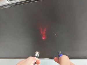
Field of view provided by the webcam was too wide in comparison to the laser spot. Ideally, the image should be less than the diameter of the laser spot. A few methods were proposed in response to this:

1. If we were unable to see the actual area, we should minimally be able to see a change in intensity of the imaged spot, with and without a magnetic sample. However, we were not able to observe such variation in intensity, probably due to the small size of the area of interest, and the weak signals we were receiving.
2. Attempted to block out all ambient light, and isolate only the signals from the laser spot, but again, we were not able to observe any obvious variation in intensity.
3. Propose the use of a beam expander before the camera - was not implemented yet.
4. Remove the blue LED about the camera which was initially there for simply aesthetics. Soldering was utilised to remove the relevant circuits and parts from the board.
5. Removed the lens in the camera, which causes the wide view.

Next: to test if LED and lens removal helped ease the situation.